

 Atoms in Motion
Matter is made of atoms
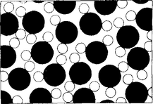
All things are made of atoms—little particles that move around in perpetual motion, attracting each other when they are a little distance apart, but repelling upon being squeezed into one another.
This is a picture of water magnified a billion times, but idealized in several ways. There are two kinds of "blobs" or circles to represent the atoms of oxygen (black) and hydrogen (white), and that each oxygen has two hydrogens tied to it. (Each little group of an oxygen with its two hydrogens is called a molecule.)
The particles are "stuck together"—that they attract each other, this one pulled by that one, etc. The whole group is "glued together," so to speak. On the other hand, the particles do not squeeze through each other. If you try to squeeze two of them too close together, they repel.
The atoms are 1 or  cm in radius. Now
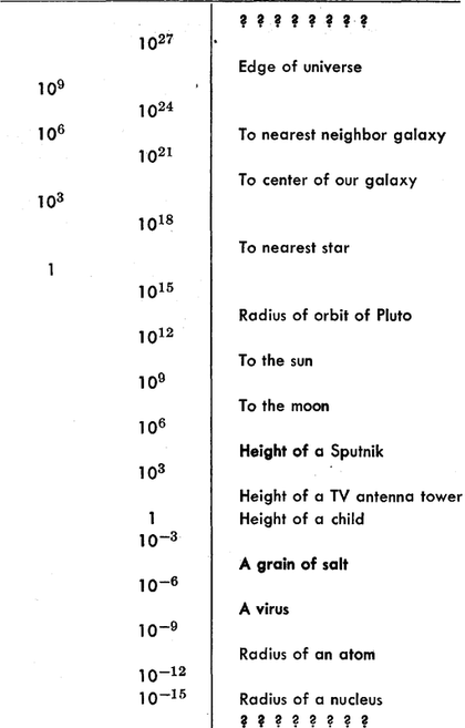
  cm is called an angstrom (just as another name), so we say they are 1 or 2 angstroms (Å) in radius. Another way to remember their size is this: if an apple is magnified to the size of the earth, then the atoms in the apple are approximately the size of the original apple.
The jiggling motion is what we represent as heat: when we increase the temperature, we increase the motion. If we heat the water, the jiggling increases and the volume between the atoms increases, and if the heating continues there comes a time when the pull between the molecules is not enough to hold them together and they do fly apart and become separated from one another. Of course, this is how we manufacture steam out of water—by increasing the temperature; the particles fly apart because of the increased motion.
At ordinary atmospheric pressure there might be only a few molecules in a whole room.
The molecules, being separated from one another, will bounce against the walls.
In order to confine a gas we must apply a pressure. The pressure times the area is the force. Clearly, the force is proportional to the area, for if we increase the area but keep the number of molecules per cubic centimeter the same, we increase the number of collisions with the piston in the same proportion as the area was increased.
Now let us put twice as many molecules in this tank, so as to double the den- sity, and let them have the same speed, i.e., the same temperature. Then, to a close approximation, the number of collisions will be doubled, and since each will be just as "energetic" as before, the pressure is proportional to the density.
If we increase the temperature without changing the density of the gas, i.e., if we increase the speed of the atoms, what is going to happen to the pressure? Well, the atoms hit harder because they are moving faster, and in addition they hit more often, so the pressure increases.
When we compress a gas slowly, the temperature of the gas increases.
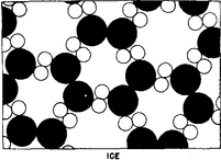
What will happen at very low temperatures is indicated in Fig. 1-4: the molecules lock into a new pattern which is ice. The interesting point is that the material has a definite place for every atom.
The difference between solids and liquids is, then, that in a solid the atoms are arranged in some kind of an array, called a crystalline array, and they do not have a random position at long distances; the position of the atoms on one side of the crystal is determined by that of other atoms millions of atoms away on the other side of the crystal.
there is a part of the symmetry that is hexagonal. You can see that if we turn the picture around an axis by 120°, the picture returns to itself. So there is a symmetry in the ice which accounts for the six-sided appearance of snowflakes. Another thing we can see from Fig. 1-4 is why ice shrinks when it melts. The particular crystal pattern of ice shown here has many "holes" in it, as does the true ice structure. When the organization breaks down, these holes can be occupied by molecules. Most simple substances, with the exception of water and type metal, expand upon melting, because the atoms are closely packed in the solid crystal and upon melting need more room to jiggle around, but an open structure collapses, as in the case of water.
Helium, even at absolute zero, does not freeze, unless the pressure is made so great as to make the atoms squash together. If we increase the pressure, we can make it solidify.
Atomics processes
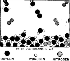
The molecules in the water are always jiggling around. From time to time, one on the surface happens to be hit a little harder than usual, and gets knocked away.
Thus, molecule by molecule, the water disappears— it evaporates. An ion is an atom which either has a few extra electrons or has lost a few electrons. In a salt crystal we find chlorine ions (chlorine atoms with an extra electron) and sodium ions (sodium atoms with one electron missing). The ions all stick together by electrical attraction in the solid salt, but when we put them in the water we find, because of the attractions of the negative oxygen and positive hydrogen for the ions, that some of the ions jiggle loose.
By equilibrium we mean that situation in which the rate at which atoms are leaving just matches the rate at which they are coming back. If there is almost no salt in the water, more atoms leave than return, and the salt dissolves. If, on the other hand, there are too many "salt atoms," more return than leave, and the salt is crystallizing.
Chemical reactions
In the case of oxygen, two oxygen atoms stick together very strongly.
Atoms are very special: they like certain particular partners, certain particular directions, and so on.
The carbon atoms are supposed to be in a solid crystal (which could be graphite or diamond*). Now, for example, one of the oxygen molecules can come over to the carbon, and each atom can pick up a carbon atom and go flying off in a new combination—"carbon-oxygen"—which is a molecule of the gas called carbon monoxide. It is given the chemical name CO.
Carbon attracts oxygen much more than oxygen attracts oxygen or carbon attracts carbon. Therefore in this process the oxygen may arrive with only a little energy, but the oxygen and carbon will snap together with a tremendous vengeance and commotion, and everything near them will pick up the energy. A large amount of motion energy, kinetic energy, is thus generated. This of course is burning.
Every substance is some type of arrangement of atoms.
We know that the carbon dioxide molecule is straight and symmetrical: O—C—O.
The most important hypothesis in all of biology, for example, is that everything that animals do, atoms do. In other words, there is nothing that living things do that cannot be understood from the point of view that they are made of atoms acting according to the laws of physics.
Basic Physics
Physics before 1920
All things, even ourselves, are made of fine-grained, enormously strongly interacting plus and minus parts, all neatly balanced out.
With this picture the atoms were easier to understand. They were thought to have a "nucleus" at the center, which is positively electrically charged and very massive, and the nucleus is surrounded by a certain number of "electrons" which are very light and negatively charged. Now we go a little ahead in our story to remark that in the nucleus itself there were found two kinds of particles, protons and neutrons, almost of the same weight and very heavy. The protons are elec- trically charged and the neutrons are neutral. If we have an atom with six protons inside its nucleus, and this is surrounded by six electrons (the negative particles in the ordinary world of matter are all electrons, and these are very light compared with the protons and neutrons which make nuclei), this would be atom number six in the chemical table, and it is called carbon. Atom number eight is called oxygen, etc., because the chemical properties depend upon the electrons on the outside, and in fact only upon how many electrons there are.
the existence of the positive charge, in some sense, distorts, or creates a "condition" in space, so that when we put the negative charge in, it feels a force. This potentiality for produc- ing a force is called an electric field. When we put an electron in an electric field, we say it is "pulled." We then have two rules: (a) charges make a field, and (b) charges in fields have forces on them and move.
Magnetic influences have to do with charges in relative motion, so magnetic forces and electric forces can really be attributed to one field, as two different aspects of exactly the same thing.
Although the forces between two charged objects should go inversely as the square of the distance, it is found, when we shake a charge, that the influence extends very much farther out than we would guess at first sight. That is, the effect falls off more slowly than the inverse square.
The only thing that is really different from one wave to another is the frequency of oscillation.
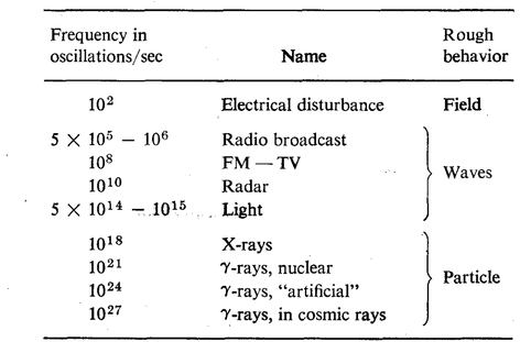
The usual "pickup" that we get from electric currents in the circuits in the walls of a building have a frequency of about one hundred cycles per second. If we increase the frequency to 500 or 1000 kilocycles (1 kilocycle = 1000 cycles) per second, we are "on the air," for this is the frequency range which is used for radio broadcasts. (Of course it has nothing to do with the air! We can have radio broadcasts without any air.) If we again increase the frequency, we come into the range that is used for FM and TV. Going still further, we use certain short waves, for example for radar. Still higher, and we do not need an instrument to "see" the stuff, we can see it with the human eye. In the range of frequency from
 to
to  cycles per second our eyes would see the oscillation of the charged comb, if we could shake it that fast, as red, blue, or violet light, depending on the frequency. Frequencies below this range are called infrared, and above it, ultraviolet. The fact that we can see in a particular frequency range makes that part of the electromagnetic spectrum no more impressive than the other parts from a physicist's standpoint, but from a human standpoint, of course, it is more interesting. If we go up even higher in frequency, we get x-rays. X-rays are nothing but very high-frequency light. If we go still higher, we get gamma rays. These two terms, x-rays and gamma rays, are used almost synonymously. Usually electromagnetic rays coming from nuclei are called gamma rays, while those of high energy from atoms are called x-rays, but at the same frequency they are indistinguishable physically, no matter what their source.
Quantum Physics
The mechanical rules of "inertia" and "forces" are wrong--Newton's laws are wrong--in the world of atoms. Instead, it was discovered that things on a small scale behave nothing like things on a large scale. That is what makes physics difficult—and very interesting. It is hard because the way things behave on a small scale is so "unnatural"; we have no direct experience with it.
Quantum mechanics has many aspects. In the first place, the idea that a particle has a definite location and a definite speed is no longer allowed; that is wrong. To give an example of how wrong classical physics is, there is a rule in quantum mechanics that says that one cannot know both where something is and how fast it is moving.
An atom has a diameter of about
cm. The nucleus has a diameter of about  cm. If we had an atom and wished to see the nucleus, we would have to magnify it until the whole atom was the size of a large room, and then the nucleus would be a bare speck which you could just about make out with the eye, but very nearly all the weight of the atom is in that infinitesimal nucleus. What keeps the electrons from simply falling in? This principle: If they were in the nucleus, we would know their position precisely, and the uncertainty principle would then require that they have a very large (but uncertain) momentum, i.e., a very large kinetic energy. With this energy they would break away from the nucleus. They make a compromise: they leave them- selves a little room for this uncertainty and then jiggle with a certain amount of minimum motion in accordance with this rule.
 There is no distinction between a wave and a particle. So quantum mechanics unifies the idea of the field and its waves, and the particles, all into one. Now it is true that when the frequency is low, the field aspect of the phenomenon is more evident, or more useful as an approximate description in terms of everyday experiences. But as the frequency increases, the particle aspects of the phenomenon become more evident with the equipment with which we usually make the measurements.
We have a new kind of particle to add to the electron, the proton, and the neutron. That new particle is called a photon. The new view of the interaction of electrons and protons that is electromagnetic theory, but with everything quantum-mechanically correct, is called quantum electrodynamics. This fundamental theory of the interaction of light and matter, or electric field and charges, is our greatest success so far in physics. In this one theory we have the basic rules for all ordinary phenomena except for gravitation and nuclear processes. For example, out of quantum electro- dynamics come all known electrical, mechanical, and chemical laws: the laws for the collision of billiard balls, the motions of wires in magnetic fields, the specific heat of carbon monoxide, the color of neon signs, the density of salt, and the reactions of hydrogen and oxygen to make water are all consequences of this one law.
Quantum electrodynamics tells the properties of very high-energy photons, gamma rays, etc. It predicted another very re- markable thing: besides the electron, there should be another particle of the same mass, but of opposite charge, called a positron, and these two, coming to- gether, could annihilate each other with the emission of light or gamma rays. (After all, light and gamma rays are all the same, they are just different points on a frequency scale.) The generalization of this, that for each particle there is an antiparticle, turns out to be true. In the case of electrons, the antiparticle has another name—it is called a positron, but for most other particles, it is called anti- so-and-so, like antiproton or antineutron.
Nuclei and particles
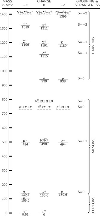
One such chart of the new particles was made independently by Gell-Mann in the U.S.A. and Nishijima in Japan. The basis of their classification is a new number, like the electric charge, which can be assigned to each particle, called its "strangeness," S. This number is conserved, like the electric charge, in reactions which take place by nuclear forces.
In Table 2-2 are listed all the particles. We cannot discuss them much at this stage, but the table will at least show you how much we do not know. Under- neath each particle its mass is given in a certain unit, called the Mev. One Mev is equal to  gram. The reason this unit was chosen is historical, and we shall not go into it now. More massive particles are put higher up on the chart; we see that a neutron and a proton have almost the same mass. In vertical columns we have put the particles with the same electrical charge, all neutral objects in one column, all positively charged ones to the right of this one, and all negatively charged objects to the left.
Particles are shown with a solid line and "resonances" with a dashed one.
Although all of the particles except the electron, neutrino, photon, graviton, and proton are unstable, decay products have been shown only for the resonances. Strangeness assignments are not applicable for leptons, since they do not interact strongly with nuclei.
All particles which are together with the neutrons and protons are called baryons,
In addition to the baryons the other particles which are involved in the nuclear interaction are called mesons. There are first the pions, which come in three varie- ties, positive, negative, and neutral; they form another multiplet.
we are confronted with a large number of particles, which together seem to be the fundamental constituents of matter. Fortunately, these particles are not all different in their interactions with one another. In fact, there seem to be just four kinds of interaction between particles which, in the order of decreasing strength, are the nuclear force, electrical interactions, the beta-decay interaction,< and gravity. The photon is coupled to all charged particles and the strength of the interaction is measured by some number, which is 1/137. The detailed law of this coupling is known, that is quantum electrodynamics. •
* The "strength" is a dimensionless measure of the coupling constant involved in each interaction.
Gravity is coupled to all energy, but its coupling is extremely weak, much weaker than that of elec- tricity. This law is also known. Then there are the so-called weak decays— beta decay, which causes the neutron to disintegrate into proton, electron, and neutrino, relatively slowly. This law is only partly known. The so-called strong interaction, the meson-baryon interaction, has a strength of 1 in this scale, and the law is completely unknown, although there are a number of known rules, such as that the number of baryons does not change in any reaction.
Elementary Interactions
Coupling Strength*
Gravity 
Weak decays 
Electromagnetic 
Mesons-baryons 1
The relation of physics to other sciences
Biology
If we have one substance and another very similar substance, the one does not just turn into the other, because the two forms are usually separated by an energy barrier or "hill." Consider this analogy: If we wanted to take an object from one place to another, at the same level but on the other side of a hill, we could push it over the top, but to do so requires the addition of some energy. Thus most chemical reactions do not occur, because there is what is called an activa- tion energy in the way. In order to add an extra atom to our chemical requires that we get it close enough that some rearrangement can occur; then it will stick. But if we cannot give it enough energy to get it close enough, it will not go to com- pletion, it will just go part way up the "hill" and back down again. However, if we could literally take the molecules in our hands and push and pull the atoms around in such a way as to open a hole to let the new atom in, and then let it snap back, we would have found another way, around the hill, which would not require extra energy, and the reaction would go easily. Now there actually are, in the cells, very large molecules, much larger than the ones whose changes we have been de- scribing, which in some complicated way hold the smaller molecules just right, so that the reaction can occur easily. These very large and complicated things are called enzymes. (They were first called ferments, because they were originally discovered in the fermentation of sugar. In fact, some of the first reactions in the cycle were discovered there.) In the presence of an enzyme the reaction will go.
An enzyme is made of another substance called protein. Enzymes are very big and complicated, and each one is different, each being built to control a certain special reaction.
We emphasize that the enzymes themselves are not involved in the reaction directly. They do not change; they merely let an atom go from one place to another. Having done so, the enzyme is ready to do it to the next molecule, like a machine in a factory.
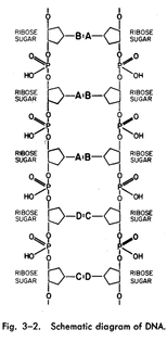
All proteins are not enzymes, but all enzymes are proteins. However, proteins are a very characteristic substance of life: first of all they make up all the enzymes, and second, they make up much of the rest of living material. Proteins have a very interesting and simple structure. They are a series, or chain, of different ammo acids. There are twenty different amino acids, and they all can combine with each other to form chains in which the backbone is CO-NH, etc. Proteins are nothing but chains of various ones of these twenty aminoacids. Each of the amino acids probably serves some special purpose. A red-eyed fly makes a red-eyed fly baby, and so the information for the whole pattern of enzymes to make red pigment must be passed from one fly to the next. This is done by a substance in the nucleus of the cell, not a protein, called DNA (short for des- oxyribose nucleic acid). This is the key substance which is passed from one cell to another (for instance, sperm cells consist mostly of DNA) and carries the information as to how to make the enzymes. DNA is the "blueprint."
The DNA molecule is a pair of chains, twisted upon each other. The backbone of each of these chains, which are analogous to the chains of proteins but chemically quite different, is a series of sugar and phosphate groups, as shown in Fig. 3-2. Now we see how the chain can contain instructions, for if we could split this chain down the middle, we would have a series BAADC . . . and every living thing could have a different series. Thus perhaps, in some way, the specific instructions for the manufacture of pro-teins are contained in the specific series of the DNA.
there are four kinds, called adenine, thymine, cytosine, and guanine, but let us call them A, B, C, and D. The interesting thing is that only certain pairs can sit opposite each other, for example A with B and C with D.
Conservation of energy
What is energy
 . There are two other conservation laws which are analogous to the conservation of energy. One is called the conservation of linear momentum. The other is called the conservation of angular momentum.
In quantum mechanics it turns out that the conservation of energy is very closely related to another important property of the world, things do not depend on the absolute time. We can set up an experiment at a given moment and try it out, and then do the same experiment at a later moment, and it will behave in exactly the same way. Whether this is strictly true or not, we do not know. If we assume that it is true, and add the principles of quantum mechanics, then we can deduce the principle of the conservation of energy. The other conservation laws are also linked together. The conservation of momentum is associated in quantum mechanics with the proposition that it makes no difference where you do the experiment, the results will always be the same. As independence in space has to do with the conservation of momentum, independence of time has to do with the conservation of energy, and finally, if we turn our apparatus, this too makes no difference, and so the invariance of the world to angular orientation is related to the conservation of angular momentum. Besides these, there are three other conservation laws, that are exact so far as we can tell today, which are much simpler to understand because they are in the nature of counting blocks.
The first of the three is the conservation of charge, and that merely means that you count how many positive, minus how many negative electrical charges you have, and the number is never changed. You may get rid of a positive with a negative, but you do not create any net excess of positives over negatives. Two other laws are analogous to this one—one is called the conservation of baryons. There are a number of strange particles, a neutron and a proton are examples, which are called baryons. In any reaction whatever in nature, if we count how many baryons are coming into a process, the number of baryons which come out will be exactly the same. There is another law, the conservation of leptons. We can say that the group of particles called leptons are: electron, mu meson, and neutrino. There is an antielectron which is a positron, that is, a −1 lepton. Counting the total number of leptons in a reaction reveals that the number in and out never changes, at least so far as we know at present.
Time and Distance
Motion
Galileo's first experiments on motion were done by using his pulse to count off equal in- tervalsoftime. Letusdothesame.
We may count off beats of a pulse as the ball rolls down the track: "one .. . two ... three .. . four .. . five ... six ... seven . . . eight..." We ask a friend to make a small mark at the location of the ball at each count; we can then measure the distance the ball travelled from the point of release in one, or two, or three, etc., equal intervals of time. Galileo expressed the result of his observations in this way: if the location of the ball is marked at 1, 2, 3, 4,... units of time from the instant ofIts release, those marks are distant from the starting point in propor- tion to the numbers 1, 4, 9, 16, ... Today we would say the distance is proportional to the square of the time:
Time
Webster defines "a time" as "a period," and the latter as "a time".
Maybe it is just as well if we face the fact that time is one of the things we probably cannot define (in the dictionary sense), and just say that it is what we already know it to be:
What really matters anyway is not how we define time, but how we measure it.
We can just say that we base our definition of time on the repetition of some apparently periodic event.
Short times
Galileo decided that a given pendulum always swings back and forth in equal intervals of time so long as the size of the swing is kept small.
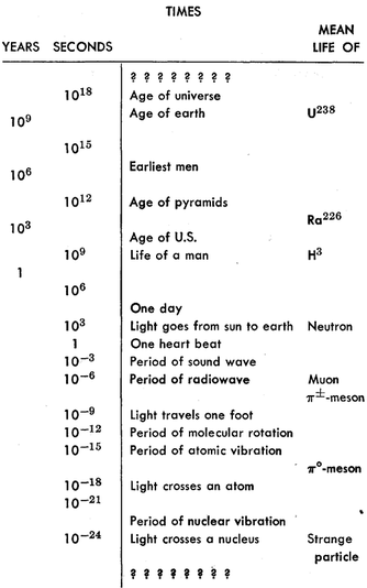
With modern electronic techniques, oscillators have been built with periods as short as about 10^-12 second, and they have been calibrated (by comparison methods such as we have described) in terms of our standard unit of time, the second.
Within the past few years, just such a technique was used to measure the lifetime of the π°-meson. By observing in a microscope the minute tracks left in a photographic emulsion in which π°-mesons had been created one saw that a π°-meson (known to be travelling at a certain speed nearly that of light) went a distance of about  meter, on the average, before disintegrating. It lived for only about
  sec.
sec.
Long times
We find that the radioactivity of a particular sample of material decreases by the same fraction for successive equal increases in its age.
We observe that if the radioactivity decreases to one-half in T days (called the "half-life"), then it decreases to one-quarter in another T days, and so on.
If we knew that a piece of material, say a piece of wood, had contained an amount A of radioactive material when it was formed, and we found out by a direct measurement that it now contains the amount B, we could compute the age of the object, t, by solving the equation
![[ {B over A}=2^{-t/T } ]](http://tlonworld.com/wp-content/ql-cache/quicklatex.com-4077a807e9285274b1ec6585b93fbe82_l3.svg "Rendered by QuickLaTeX.com")
There are, fortunately, cases in which we can know the amount of radioactivity that was in an object when it was formed. We know, for example, that the carbon dioxide in the air contains a certain small fraction of the radioactive carbon isotope C14 (replenished continuously by the action of cosmic rays). If we measure the total carbon content of an object, we know that a certain fraction of that amount was originally the radioactive C14; we know, therefore, the starting amount A to use in the formula above. Carbon-14 has a half-life of 5000 years. By careful measurements we can measure the amount left after 20 half-lives or so and can therefore "date" organic objects which grew as long as 100,000 years ago.
Uranium, for example, has an isotope whose half-life is about 109 years, so that if some material was formed with uranium in it 10^9 years ago, only half the uranium would remain today. When the uranium disintegrates, it changes into lead. Consider a piece of rock which was formed a long time ago in some chemical process. Lead, being of a chemical nature different from uranium, would appear in one part of the rock and uranium would appear in another part of the rock. The uranium and lead would be separate. If we look at that piece of rock today, where there should only be uranium we will how find a certain fraction of uranium and a certain fraction of lead. By comparing these fractions, we can tell what percent of the uranium disappeared and changed into lead. By this method, the age of certain rocks has been determined to be several billion years.
It is now believed that at least our part of the universe had its beginning about ten or twelve billion years ago.
Units and standards of time
Recently we have been gaining experience with some natural oscillators which we now believe would provide a more constant time reference than the earth, and which are also based on a natural phenomenon available to everyone. These are the so-called "atomic clocks." Their basic internal period is that of an atomic vibration which is very insensitive to the temperature or any other external effects. These clocks keep time to an accuracy of one part in  or better.
Large distances
We have found by experience that dis- tance can be measured in another fashion: by triangulation.
For example, we were able to use triangulation to measure the height of the first Sputnik. We found that it was roughly  meters high. By more careful measurements the distance to the moon can be measured in the same way. Two telescopes at different places on the earth can give us the two angles we need. It has been found in this way that the moon is
  meters away.
because the earth moving around the sun gives us a large baseline for measurements of objects outside the solar system. If we focus a telescope on a star in summer and in winter, we might hope to determine these two angles accurately enough to be able to measure the distance to a star.
Astronomers are always inventing new ways of measuring distance. They find, for example, that they can estimate the size and brightness of a star by its color. The color and brightness of many nearby stars—whose distances are known by triangula- tion—have been measured, and it is found that there is a smooth relationship between the color and the intrinsic brightness of stars (in most cases). If one now measures the color of a distant star, one may use the color-brightness relationship to determine the intrinsic brightness of the star. By measuring how bright the star appears to us at the earth (or perhaps we should say how dim it appears), we can compute how far away it is. (For a given intrinsic brightness, the apparent brightness decreases with the
square of the distance.). Evidence supports the idea that galaxies are all about the same size.
Photographs of exceedingly distant galaxies have recently been obtained with the giant Palomar telescope. One is shown in Fig. 5-8. It is now believed that some of these galaxies are about halfway to the limit of the universe— meters away—the largest distance we can contemplate!
Short distances
With- out much difficulty we can mark off one thousand equal spaces which add up to one meter. With somewhat more difficulty, but in a similar way (using a good microscope), we can mark off a thousand equal subdivisions of the millimeter to make a scale of microns (millionths of a meter). It is difficult to continue to smaller scales, because we cannot "see" objects smaller than the wavelength of visible light (about  meter).
from an observation of the way light of short wavelength (x-radiation) is reflected from a pattern of marks of known separation, we determine the wave- length of the light vibrations. Then, from the pattern of the scattering of the same light from a crystal, we can determine the relative location of the atoms in the crystal, obtaining results which agree with the atomic spacings also determined by chemical means. We find in this way that atoms have a diameter of about  meter.
Measurement of a nuclear cross section can be made by passing a beam of high-energy particles through a thin slab of material and observing the number of particles which do not get through.
The chance that a very small particle will hit a nucleus on the trip through is just the total area covered by the profiles of the nuclei divided by the total area in the picture. Suppose that we know that in an area A of our slab of material there are N atoms (each with one nucleus, of course). Then the total area "covered" by the nuclei is  . Now let the number of particles of our beam which arrive
at the slab be  and the number which come out the other side be
  . The fraction which do not get through is
  which should just equal the fraction of the area covered. We can obtain the radius of the nucleus from the equation
![[ sigma=pi r^2={Aover N}left( 1-{n_2over n_1} right) ]](http://tlonworld.com/wp-content/ql-cache/quicklatex.com-0df635738b182ca6ddd048c464dbba4f_l3.svg "Rendered by QuickLaTeX.com")
From such an experiment we find that the radii of the nuclei are from about 1 to 6 times  meter. The length unit meter is called the fermi, in honor of Enrico Fermi (1901-1958).
It might be thought that it would be a good idea to use some natural length as our unit of length—say the radius of the earth or some fraction of it. The meter was originally intended to be such a unit and was defined to be  times the earth's radius.
Perfectly precise measurements of distances or times are not permitted by the laws of nature. We have mentioned earlier that the errors in a measurement of the position of an object must be at least as large as
![[ Delta xge hbar /2 Delta p ]](http://tlonworld.com/wp-content/ql-cache/quicklatex.com-f4a21e108da026f21f9d1be604a6d7ce_l3.svg "Rendered by QuickLaTeX.com")
where  is a small quantity called "Planck's constant" and ∆p is the error in our knowledge of the momentum (mass times velocity) of the object whose posi- tion we are measuring. It was also mentioned that the uncertainty in position measurements is related to the wave nature of particles.
The relativity of space and time implies that time measurements have also a minimum error, given in fact by
![[ Delta tge hbar/2 Delta E, ]](http://tlonworld.com/wp-content/ql-cache/quicklatex.com-81ac1f059de822f126e0548271081efc_l3.svg "Rendered by QuickLaTeX.com")
where ΔE is the error in our knowledge of the energy of the process whose time period we are measuring. If we wish to know more precisely when something happened we must know less about what happened, because our knowledge of the energy involved will be less. The time uncertainty is also related to the wave nature of matter.
Probability
Chance and likelihood
 Let us designate the two outcomes by W (for "win") and L (for "lose"). In the general case, the probability of W or Lin a single event need not be equal. Let p be the probability of obtaining the result W. Then q, the probability of L, is necessarily (1-p). In a set of n trials, the probability P(k, n) that W will be obtained k times is
 ![[ P(k,n)={n! over k! (n-k)!} , p^k , q^{n-k} ]](http://tlonworld.com/wp-content/ql-cache/quicklatex.com-d43664dcc964a44d3bacf2d9deabea56_l3.svg "Rendered by QuickLaTeX.com")
 is positive for either positive or negative motion, and is therefore a reasonable measure of such random wandering.
 We can show that the expected value of
 is just N, the number of steps taken. By "expected value" we mean the probable value (our best guess), which we can think of as the expected average behavior in many repeated sequences. We represent such an expected value by <>, and may refer to it also as the "mean square distance." After one step, is always +1, so we have certainly
  . (All distances will be measured in terms of a unit of one step. We shall not continue to write the units of distance.)
 The expected value of
 for N > 1 can be obtained from
  .
. After N steps we have
![[ D_N^2= (D_{N-1}+1)^2 quad {rm or} quad (D_{N-1}-1)^2 ]](http://tlonworld.com/wp-content/ql-cache/quicklatex.com-dea3ea099d4b0b5ca53d24747188d08b_l3.svg "Rendered by QuickLaTeX.com")
The average expectation is then 
 or, equivalently, the "root means square
  . Our derivation for
  would proceed as before except that Eq. (6.8) would be changed now to read
 ![[ langle D_N^2 rangle =langle D_{N-1}^2 rangle +langle S^2 rangle =langle D_{N-1}^2 rangle +1=N ]](http://tlonworld.com/wp-content/ql-cache/quicklatex.com-65aac674672eb1a3df540f3e1d74c46c_l3.svg "Rendered by QuickLaTeX.com")
We expect that for small ∆x the chance of D landing in the interval is proportional to ∆x, the width of the interval. So we can write
P(x, ∆x) = p(x) ∆x
The function p(x) is called the probability density.
For large N, p(x) is the same for all reasonable distributions in individual step lengths, and depends only on N. We plot p(x) for three values of N in Fig. 6-7. You will notice that the "half-widths" (typical spread from x = 0) of these curves is
 , as we have shown it should be.
 You may notice also that the value of p(x) near zero is inversely proportional to
. This comes about because the curves are all of a similar shape and their areas under the curves must all be equal. The normal or gaussian probability density. It has the mathematical form
![[ p(x)={e^{-x^2over 2sigma^2}over sigma sqrt{2pi}}]](http://tlonworld.com/wp-content/ql-cache/quicklatex.com-004fdfa40fd6145a9ce4010f5630ff03_l3.svg "Rendered by QuickLaTeX.com")
where σ is called the standard deviation and is given, in our case, by  .
.
We remarked earlier that the motion of a molecule, or of any particle, in a gas is like a random walk. Suppose we open a bottle of an organic compound and let some of its vapor escape into the air. If there are air currents, so that the air is circulating, the currents will also carry the vapor with them. But even in perfectly still air, the vapor will gradually spread out-will diffuse-until it has penetrated throughout the room. We might detect it by its color or odor. The individual molecules of the organic vapor spread out in still air because of the molecular motions caused by collisions with other molecules. If we know the average "step" size, and the number of steps taken per second, we can find the probability that one, or several, molecules will be found at some distance from their starting point after any particular passage of time.
The motion of a molecule, or of any particle, in a gas is like a random walk. Suppose we open a bottle of an organic compound and let some of its vapor escape into the air. If there are air currents, so that the air is circulating, the currents will also carry the vapor with them. But even in perfectly still air, the vapor will gradually spread out-will diffuse-until it has penetrated throughout the room. We might detect it by its color or odor. The individual molecules of the organic vapor spread out in still air because of the molecular motions caused by collisions with other molecules. If we know the average "step" size, and the number of steps taken per second, we can find the probability that one, or several, molecules will be found at some distance from their starting point after any particular passage of time.
The uncertainty principle
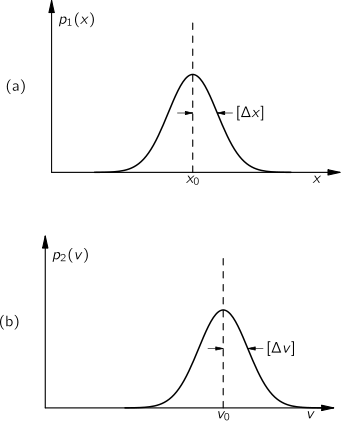
 , such that is the probability that the particle will be found between x and x +∆x If the particle is reasonably well localized, say near
  , the function might be given by the graph of Fig. 6-lO(a). Similarly, we must specify the velocity of the particle by means of a probability density
  , with the probability that the velocity will be found between v and v +∆v
It is one of the fundamental results of quantum mechanics that the two functions
and cannot be chosen independently and, in particular, cannot both be made arbitrarily narrow. If we call the typical "width" of the curve  and that of the curve ∆v, nature demands that the product of the two widths be at least as big as the number
  , where m is the mass of the particle and his a fundamental physical constant called Planck's constant. We may write this basic relationship as
 ![[ langle Delta x rangle langle Delta x rangle geq hbar /2m ]](http://tlonworld.com/wp-content/ql-cache/quicklatex.com-5c13fccbb04c2f0a33f5ac6f9515a52c_l3.svg "Rendered by QuickLaTeX.com")
This equation is a statement of the Heisenberg uncertainty principle.
This equation says that if we try to "pin down" a particle by forcing it to be at a particular place, it ends up by having a high speed. Or if we try to force it to go very slowly, or at a precise velocity, it "spreads out" so that we do not know very well just where it is.
The necessary uncertainty in our specification of the position of a particle becomes most important when we wish to describe the structure of atoms. In the hydrogen atom, which has a nucleus of one proton with one electron outside of the nucleus, the uncertainty in the position of the electron is as large as the atom itself! Wecannot,therefore,properlyspeakoftheelectronmovinginsome"orbit" around the proton. The most we can say is that there is a certain chance p(r) ΔV, of observing the electron in an element of volume V at the distance r from the proton. The probability density p(r) is given by quantum mechanics. For an undisturbed hydrogen atom  , which is a bell-shaped function like that in Fig. 6-8. The number a is the "typical" radius, where the function is decreasing rapidly. Since there is a small probability of finding the electron at distances from the nucleus much greater than a, we may think of a as "the radius of the atom," about 10^-10 meter.
Our best "picture" of a hydrogen atom is a nucleus surrounded by an "electron cloud" (although we really mean a "probability cloud"). The electron is there somewhere, but nature per- mits us to know only the chance of finding it at any particular place.
 The Theory of Gravitation
Planetary motion
Every object in the universe attracts every other object with a force which for any two bodies is proportional to the mass of each and varies inversely as the square of the distance between them. This state- ment can be expressed mathematically by the equation
![[ F={ G m m' over r^2} ]](http://tlonworld.com/wp-content/ql-cache/quicklatex.com-5c0d0f638b71e78ae4f8f8e47054942e_l3.svg "Rendered by QuickLaTeX.com")
An object responds to a force by accelerating in the direction of the force by an amount that is inversely proportional to the mass of the object.Tycho Brahe had an idea that was different from anything proposed by the ancients: his idea was that these debates about the nature of the motions of the planets would best be resolved if the actual positions of the planets in the sky were measured sufficiently accurately. If measurement showed exactly how the planets moved, then perhaps it would be possible to establish one or another viewpoint. This was a tremendous idea-that to find something out, it is better to perform some careful experiments than to carry on deep philosophical arguments. Pursuing this idea, Tycho Brahe studied the positions of the planets for many years in his observatory on the island of Hven, near Copenhagen. He made voluminous tables, which were then studied by the mathematician Kepler, after Tycho's death.
Kepler's laws
I. Each planet moves around the sun in an ellipse, with the sun at one focus.
II. The radius vector from the sun to the planet sweeps out equal areas in equal intervals of time.
III. The squares of the periods of any two planets are proportional to the cubes of the semimajor axes of their respective orbits:
 .
. Development of dynamics
Newton modified this idea, saying that the only way to change the motion of a body is to use force.
For example, if a stone is attached to a string and is whirling around in a circle, it takes a force to keep it in the circle. We have to pull on the string. In fact, the law is that the acceleration produced by the force is inversely proportional to the mass, or the force is proportional to the mass times the acceleration. The more massive a thing is, the stronger the force required to produce a given acceleration.
Newton's laws of gravitation
There must be a force, inversely as the square of the distance, directed in a line between the two objects.
Being a man of considerable feeling for generalities, Newton supposed, of course, that this relationship applied more generally than just to the sun holding the planets. It was already known, for example, that the planet Jupiter had moons going around it as the moon of the earth goes around the earth, and Newton felt certain that each planet held its moons with a force. He already knew of the force holding us on the earth, so he proposed that this was a universal force- that everything pulls everything else.
We can calculate from the radius of the moon's orbit (which is about 240,000 miles) and how long it takes to go around the earth (approximately 29 days), how far the moon moves in its orbit in 1 second, and can then calculate how far it falls in one second.* This distance turns out to be roughly 1/20 of an inch in a second.
Wishing to put this theory of gravitation to a test by similar calculations, Newton made his calculations very carefully and found a discrepancy so large that he regarded the theory as contradicted by facts, and did not publish his results. Six years later a new measurement of the size of the earth showed that the astronomers had been using an incorrect distance to the moon. When Newton heard of this, he made the calculation again, with the corrected figures, and obtained beautiful agreement.
the moon falls in the sense that it falls away from the straight line that it would pursue if there were no forces. Let us take an example on the surface of the earth. An object released near the earth's surface will fall 16 feet m the first second. An obJect shot out horizontally will also fall 16 feet; even though it is movmg honzontally, it still falls the same 16 feet in the same time.
if the bullet moves at 5 miles a second, it then will continue to fall toward the earth at the same rate of 16 feet each second, but will never get any closer because the earth keeps curving away from it.
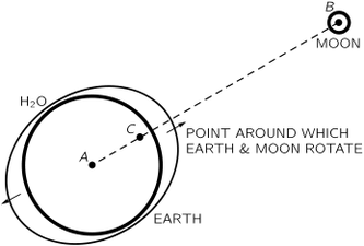
the pull of the moon for the earth and for the water is "balanced" at the center. But the water which is closer to the moon is pulled more than the average and the water which is farther away from it is pulled less than the average. Furthermore, the water can flow while the more rigid earth cannot. The true picture is a combination of these two things.
the earth and the moon both go around a central position, each falling toward this common position, as shown in Fig. 7-5. This motion around the common center is what balances the fall of each. So the earth is not going in a straight hoe either; 1t travels in a circle. The water on the far side is "unbalanced" because the moon's attraction there is weaker than 1t is at the cemer of the earth, where it JUSt balances the "centnfugal force." The result of this imbalance 1s that the water rises up, away from the center of the earth. On the near side, the attrac- tion from the moon is stronger, and the imbalance is in the opposite direction m space, but agam away from the center of the earth. The net result 1s that we get two tidal bulges.
Universal gravitation
there was once a certain difficulty with the moons of Jupiter that is worth remarking on. These satellites were studied very carefully by Roemer, who noticed that the moons sometimes seemed to be ahead of schedule, and some- times behind. (One can find their schedules by waiting a very long time and finding out how long it takes on the average for the moons to go around.) Now they were ahead when Jupiter was particularly close to the earth and they were behind when Jupiter wasfarther from the earth. This would have been a very difficult thing to explain according to the law of gravitation-it would have been, in fact, the death ofthiswonderfultheoryiftherewerenootherexplanation. Ifalawdoesnotwork even in one place where it ought to, it is just wrong. But the reason for this dis- crepancy was very simple and beautiful: it takes a little while to see the moons of Jupiter because of the time it takes light to travel from Jupiter to the earth. When Jupiter is closer to the earth the time is a little less, and when it is farther from the earth, the time is more. This is why moons appear to be, on the average, a little ahead or a little behind, depending on whether they are closer to or farther from the earth. This phenomenon showed that light does not travel instantaneously, and furnished the first estimate of the speed of light. This was done in 1656.
Attempts were made to analyze the motions of Jupiter, Saturn, and Uranus on the basis of the law of gravitation. The effects of each of these planets on each other were calculated to see whether or not the tiny deviations and irregularities in these motions could be completely understood from this one law. Lo and behold, for Jupiter and Saturn, all was well, but Uranus was "weird." It behaved in a very peculiar manner. It was not travelling in an exact ellipse, but that was under- standable, because of the attractions of Jupiter and Saturn. But even if allowance were made for these attractions, Uranus still was not going right, so the laws of gravitation were in danger of being overturned, a possibility that could not be ruled out. Two men, Adams and Leverrier, in England and France, independently, arrived at another possibility: perhaps there is another planet, dark and invisible, which men had not seen. This planet, N, could pull on Uranus. They calculated where such a planet would have to be in order to cause the observed perturba- tions. They sent messages to the respective observatories, saying, "Gentlemen, point your tekscope to such and such a place, and you will see a new planet." It often depends on with whom you are working as to whether they pay any atten- tion to you or not. They did pay attention to Leverrier; they looked, and there planet N was! The other observatory then also looked very quickly in the next few days and saw it too.
Cavendish's experiemnt
All the masses and distances are known. You say, "We knew it already for the earth." Yes, but we did not know the mass of the earth. By knowing G from this experiment and by knowing how strongly the earth attracts, we can indirectly learnhowgreatisthemassoftheearth! Thisexperimenthasbeencalled"weighing the earth." Cavendish claimed he was weighing the earth, but what he was meas- uring was the coefficient G of the gravity law. This is the only way in which the mass of the earth can be determined. G turns out to be
 newton·
  .
. . The question is, where does such a large number come from?
 let us consider the time it takes light to go across a proton,
 second. If we compare this time with the age of the universe,
  years, the answer is
  . It has about the same number.
It is very interesting that this force is exactly proportional to the mass with great precision, because if it were not exactly proportional there would be some effect by which inertia and weight would differ. The absence of such an effect has been checked with great accuracy by an experiment done first by Eotvos in 1909 and more recently by Dicke. For all substances tried, the masses and weights are exactly proportional within I part m 1,000,000,000, or less. This is a remarkable experiment.
Gravity and relativity

Newton's laws of dynamics
Momentum and forces
Galileo made a great advance in the understanding of motion when he discovered the principle of tnertia: If an object is left alone, is not disturbed, it continues to move with a constant velocity in a straight line if it was originally moving, or it continues to stand still if it was just standing still.
Newton wrote down three laws: The First Law was a mere restatement of the Galilean principle of inertia just described. The Second Law gave a specific way of determinmg how the velocity changes under different influences called forces. The Third Law describes the forces to some extent.
We use the term mass as a quantitative measure of inertia, and we may measure mass, for example, by swmgmg an object in a circle at a certain speed and measuring how much force we need to keep it in the circle. In this way we find a certain quantity of mass for every object. Now the momentum of an object is a product of two parts: its mass and its velocity. Thus Newton's Second Law may be written mathematically this way:
![[ F ={ d over dt} (mv). ]](http://tlonworld.com/wp-content/ql-cache/quicklatex.com-fe7f55ea4ddcbec6e4337e90e0ead010_l3.svg "Rendered by QuickLaTeX.com")
The time-rate-of-change of a quantity called momentum is proportional to the force. For a constant mass
![[ F=m {dv over dt} =m, a ]](http://tlonworld.com/wp-content/ql-cache/quicklatex.com-24b6d9d73d423770ea0bab41016cbfcc_l3.svg "Rendered by QuickLaTeX.com")
The acceleration a is the rate of change of the velocity.
An object moving in a circle of radius R with a certain speed v along the circle falls away from a straightline path by a distance equal to  if t is very small. Thus the formula for acceleration at right angles to the motion is
  and a force F at right angles to the velocity will cause an object to move in a curved path whose radius of curvature is
  .
.
Newton third law
Action equals reaction. Suppose we have two small bodies, say particles, and suppose that the first one exerts a force on the second one, pushing it with a certain force. Then, simultaneously, according to Newton's Third Law, the second particle will push on the first with an equal force, in the opposite direction; furthermore, these forces effectively act in the same line.
Conservation of momentum
Suppose, for simplicity, that we have just two interacting particles, possibly of different mass, and numbered I and 2. The forces between them are equal and opposite; what are the consequences? According to Newton's Second Law, force is the time rate of change of the momentum, so we conclude that the rate of change of momentum  of particle I is equal to minus the rate of change of momentum
  of particle 2. This means that if we add the momentum of particle I to the momentum of particle 2, the rate of change of the sum of these, due to the mutual forces (called internal forces) between particles, is zero
  .
.
There is another interesting consequence of Newton's Second Law, to be proved later, but merely stated now. This principle is that the laws of physics will look the same whether we are standing still or moving with a uniform speed in a straight line.
Relativistic momentum
In the theory of relativity it turns out that we do have conservation of momentum; the particles have mass and the momentum is still given by mv, the mass times the velocity, but the mass changes with the velocity, hence the momentum also changes. The mass varies with velocity according to the law
![[ m={ m_0 over sqrt{1-{v^2 over c^2}} ]](http://tlonworld.com/wp-content/ql-cache/quicklatex.com-4c7f64cd778283eeeb00ec47205d6157_l3.svg "Rendered by QuickLaTeX.com")
where m0 is the mass of the body at rest and c is the speed of light. It is easy to see from the formula that there is negligible difference between m and m0 unless v is very large, and that for ordinary velocities the expression for momentum reduces to the old formula.
If an electrical charge at one location is suddenly moved, the effects on another charge, at another place, do not appear instantane- ously-there is a little delay.
It takes time for the influence to cross the intervening distance, which it does at 186,000 miles a second. In that tiny time themomentumoftheparticlesisnotconserved. Ofcourseafterthesecondcharge has felt the effect of the first one and all is quieted down, the momentum equation will check out all right, but during that small interval momentum is not conserved. We represent this by saying that during this interval there is another kind of mo- mentum besides that of the particle, ml!, and that is momentum in the electro- magnetic field. If we add the field momentum to the momentum of the particles, then momentum is conserved at any moment all the time.
To take another example: an electromagnetic field has waves, which we call light; it turns out that light also carries momentum with it, so when light impinges on an object it carries in a certain amount of momentum per second; this is equivalent to a force, because if the illuminated object is picking up a certain amount of momentum per second, its momentum is changing and the situation is exactly the same as if there were a force on it.
In quantum mechanics the difference is that when the particles are represented as particles, the momentum is still mv, but when the particles are represented as waves, the momentum is measured by the number of waves per centimeter: the greater this number of waves, the greater the momen- tum. In spite of the differences, the law of conservation of momentum holds also in quantum mechanics.
Symmetry in Physics
Professor Hermann Weyl has given this definition of symmetry: a thing is symmetrical if one can subject it to a certain operation and it appears exactly the same after the operation.
The laws of physics are symmetrical for translational displacements and rotations. It should make no difference in which direction we choose the axes.
 Characteristic of forces
Friction
The frictional force is proportional to the normal force, and has a more or less constant coefficient; that is,
F=μN
where μ is called the coefficient of friction. The coefficient of friction is independent of the weight.
That the formula F=μN is approximately correct can be demonstrated by a simple experiment. We set up a plane, inclined at a small angle θ, and place a block of weight WW on the plane. We then tilt the plane at a steeper angle, until the block just begins to slide from its own weight. The component of the weight downward along the plane is Wsinθ , and this must equal the frictional force F when the block is sliding uniformly. The component of the weight normal to the plane is Wcosθ , and this is the normal force N. With these values, the formula becomes Wsinθ=μWcosθ , from which we get μ= tanθ. If this law were exactly true, an object would start to slide at some definite inclination. If the same block is loaded by putting extra weight on it, then, although W is increased, all the forces in the formula are increased in the same proportion, and W cancels out.
Molecular forces
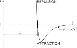
The force between atoms is illustrated schematically in the Figure, where the force F between two atoms is plotted as a function of the distance r between them. There are different cases: in the water molecule, for example, the negative charges sit more on the oxygen, and the mean positions of the negative charges and of the positive charges are not at the same point; consequently, another molecule nearby feels a relatively large force, which is called a dipole-dipole force. However, for many systems the charges are very much better balanced, in particular for oxygen gas, which is perfectly symmetrical. In this case, although the minus charges and the plus charges are dispersed over the molecule, the distribution is such that the center of the minus charges and the center of the plus charges coincide. A molecule where the centers do not coincide is called a polar molecule, and charge times the separation between centers is called the dipole moment. A nonpolar molecule is one in which the centers of the charges coincide. For all nonpolar molecules, in which all the electrical forces are neutralized, it nevertheless turns out that the force at very large distances IS an attraction and varies inversely as the seventh power of the distance, or  , where k is a constant that depends on the molecules.
Since the molecular forces attract at large distances and repel at short dis- tances, as shown in Figure, we can make up solids in which all the atoms are held together by their attractions and held apart by the repulsion that sets in when they are too close together.
Fundamental forces fields
If any two bodies are electrically charged, there is an electrical force between them, and if the magnitudes of the charges are q1 and q2, respectively, the force varies inversely as the square of the distance between the charges, or
![[ F ={ q_1, q_2over 4 pi , epsilon_0, r^2} ]](http://tlonworld.com/wp-content/ql-cache/quicklatex.com-7b622a9cec84240daafe8fd3d562af88_l3.svg "Rendered by QuickLaTeX.com")
with  . For unlike charges, this law is like the law of gravitation, but for like charges the force is repulsive and the sign (direction) is reversed.
The most important charge of all is the charge on a single electron, which is  coulomb.
The combination  occurs frequently, and to simplify calculations it has been defined by the symbol
  ; its numerical value in the mks system of units turns out to be
  . The advantage of using the constant in this form is that the force between two electrons in newtons can then be written simply as
  .
.
To analyze the force by means of the field concept, we say that the charge  at P produces a "condition" at R, such that when the charge
  is placed at R it "feels" the force. E is the "condition" produced by qb we say, and F is the response of to E. E is called an electric field, and it is a vector. In the case of gravitation, we can do exactly the same thing. The force on
  is the mass times the field C produced by
  ; that is,
  .
.
The total electric field produced by a number of sources is the vector sum of the electric fields produced by the first source, the second source, and so on.
Closely related to electrical force is another kind, called magnetic force, and this too is analyzed in terms of a field.
The first part of the experiment is to apply a negative voltage to the lower plate, which means that extra electrons have been placed on the lower plate. Since like charges repel, the light spot on the screen instantly shifts upward. (We could also say this in another way-that the electrons "felt" the field, and responded by deflecting upward.) We next reverse the voltage, making the upper plate negative. The light spot on the screen now jumps below the center, showing that the electrons in the beam were repelled by those in the plate above them. (Or we could say again that the electrons had "responded" to the field, which is now in the reverse direction.)
The second part of the experiment is to disconnect the voltage from the plates and test the effect of a magnetic field on the electron beam. This is done by means of a horseshoe magnet, whose poles are far enough apart to more or less straddle the tube. Suppose we hold the magnet below the tube in the same orienta- tion as the letter U, with its poles up and part of the tube in between. We note that the light spot is deflected, say, upward, as the magnet approaches the tube from below. So it appears that the magnet repels the electron beam. However, it is not that simple, for if we invert the magnet without reversing the poles side-for- side, and now approach the tube from above, the spot still moves upward, so the electron beam is not repelled; instead, it appears to be attracted this time. Now we start again, restoring the magnet to its original U orientation and holding it below the tube, as before. Yes, the spot is still deflected upward; but now turn the magnet ISO degrees around a vertical axis, so that it is still in the U position but the poles are reversed side-for-side. Behold, the spot now jumps downward, and stays down, even if we invert the magnet and approach from above, as before.
Across the magnet from one pole to the other there is a magnetic field. This field has a direction which is always away from one particular pole (which we could mark) and toward the other. Inverting the magnet did not change the direction of the field, but reversing the poles side-for-side did reverse its direction. For example, if the electron velocity were horizontal in the x-direction and the magnetic field were also horizontal but in they-direction, the magnetic force on the moving electrons would be in the z-direction, i.e., up or down, depending on whether the field was in the positive or negative y-direction.
The force on a charged object depends upon its motion; if, when the object is standing still at a given place, there is some force, this is taken to be proportional to the charge, the coefficient being what we call the electric field. When the object moves the force may be different, and the correction, the new "piece" of force, turns out to be dependent exactly linearly on the velocity, but at right angles to v and to another vector quantity which we call the magnetic induction B.
The total electric and magnetic force on a moving charge q has the components

Pseudo forces
The laws of force as looked upon by Moe would appear as
![[ m { d^2x' over dt^2} =F, x' - m, a ]](http://tlonworld.com/wp-content/ql-cache/quicklatex.com-4a4ad43cf33575bf2f1ac9c05d5e3f23_l3.svg "Rendered by QuickLaTeX.com")
That is, since Moe's coordinate system is accelerating with respect to Joe's.
Another example of pseudo force is what is often called "centrifugal force." An observer in a rotating coordmate system, e.g., in a rotating box, will find mysterious forces, not accounted for by any known origin of force, throwing things outward toward the walls.
One very important feature of pseudo forces is that they are always propor- tional to the masses; the same is true of gravity.
Einstein put forward the famous hypothesis that accelerations give an imita- tion of gravitation, that the forces of acceleration (the pseudo forces) cannot be distinguished from those of gravity; it is not possible to tell how much of a given force is gravity and how much is pseudo force.
Suppose that we all lived in two dimensions, and knew nothing of a third. We think we are on a plane, but suppose we are really on the surface of a sphere. And suppose that we shoot an object along the ground, with no forces on it. Where will it go? It will appear to go in a straight line, but it has to remain on the surface of a sphere, where the shortest distance between two points is along a great circle; so it goes along a great circle. If we shoot another object similarly, but in another direction, it goes along another great circle. Because we think we are on a plane, we expect that these two bodies will continue to diverge linearly with time, but careful observation will show that if they go far enough they move closer together again, as though they were attracting each other. But they are rzot attracting each other-there is just something "weird" about this geometry. This particular illustration does not describe correctly the way in which Euclid's geometry is "weird," but it illustrates that if we distort the geometry sufficiently it is possible that all gravitation is related in some way to pseudo forces; that is the general idea of the Einsteinian theory of gravitation.
Nuclear forces
Forces within a nucleus do not vary inversely as the square of the distance, but die off exponentially over a certain distance r, as expressed by
 , where the distance
  is of the order of to centimeters.
 Work and potential energy
Energy of a falling body
An object which changes its height under the influence of gravity alone has a kinetic energy T=m v^2/2 due to its motion during the fall, and a potential energy mgh, abbreviated U=mgh., whose sum is constant:
![[ T+U=m v^2/2 +m,g,h = const ]](http://tlonworld.com/wp-content/ql-cache/quicklatex.com-36788e7f35e9bdb684f2f5f959a7ff76_l3.svg "Rendered by QuickLaTeX.com")
As a result, the closer the planet is to the sun, the faster it is going. The rate of change of kinetic energy of an object zs equal to the power expended by the forces acting on it.
![[ {d Tover dt } =F, v ]](http://tlonworld.com/wp-content/ql-cache/quicklatex.com-40d96b52e111e53be5e8c7827de90d5a_l3.svg "Rendered by QuickLaTeX.com")
The work done by the force on the object is defined by the integral
![[ W=delta T=int F, ds=- Delta , V=-m, g, int dh ]](http://tlonworld.com/wp-content/ql-cache/quicklatex.com-59f2cbe29d55e2d1374438c8e4ee92af_l3.svg "Rendered by QuickLaTeX.com")
Work is measured in newton · meters. A newton-meter is called a Joule; work is measured in joules. Power, then, is joules per second, and that is also called a watt.
For example the work done by the gravity force in bringing a body from a point at a distance r1 to a point at the distance r2 is
![[ W_{12}=−int { G ,M ,m, drover r^2} =G ,M ,m, left( {1over r_2}-{1over r_1} right) ]](http://tlonworld.com/wp-content/ql-cache/quicklatex.com-28213a7a5faa75505cf0e6521c8ed3e0_l3.svg "Rendered by QuickLaTeX.com")
When there are friction forces the conservation of energy seems at first sight to be invalid. We have to find another form of energy. It turns out, in fact, that heat is generated in an object when it rubs another with friction.
Only the component of force in the direction of the displacement does any work.
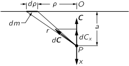
Gravitational field produced by mass distributions.
The gravitational field  produced by an infinite sheet of material with constant density of mass μ at a distance "a" is given by the integral of
  along the sheet. It points along the direction orthogonal to the sheet, let us say z, and is given by
![[ C_z =−G a int { dm over r^3} =−G a, mu ,2,pi int_{0}^infty {rho,drho over (rho^2+a^2)^{3over 2}} =−G a , mu, 2,pi ,int_{a}^infty dr/r^2=2 ,pi,mu , G ]](http://tlonworld.com/wp-content/ql-cache/quicklatex.com-6b1680f9466f8b5279a4a8d8830c25ab_l3.svg "Rendered by QuickLaTeX.com")
The force is independent of distance a!
The force produced by the earth at a point on the surface or outside it is the same as if all the mass of the earth were located at its center.
Conservative forces
In general the work depends upon the curve, but in special cases it does not. If it does not depend up011 the curve, we say that the force is a conservative force.
If only conservative forces act, the kinetic energy T plus thepotential energy U remains constant:
T + U = constant.
All the fundamental forces in nature appear to be conservative.
 The special theory of relativity
The principle of relativity
The principle of relativity was first stated by Newton, in one of his corollaries to the laws of motion: "The motions of bodies included in a given space are the same among themselves, whether that space is at rest or moves uniformly forward in a straight line."
Suppose that Moe is moving in the x-direction with a uniform velocity u, and he measures the position of a certain point. He designates the "x-distance" of the point in his coordinate system as x'. Joe is at rest, and measures the position of the same point, designating its x-coordinate in his system as x. The relationship of the coordinates in the two systems is
x'=x- ut
t'=t *
Newton's equations are invariant under these transformations. In the past century interest in it was heightened as the result of investigations into the phenomena of electricity, magnetism, and light. A long series of careful studies of these phenomena by many people culminated in Maxwell's equations of the electromagnetic field, which describe electricity, magnetism, and light in one uniform system. However, the Maxwell equations did not seem to obey the principle of relativity. That is, if we transform Maxwell's equations by the substitution of equations *, their form does not remain the same; therefore, in a moving space ship the electrical and optical phenomena should be different from those in a stationary ship.
Suppose we are riding in a car that is going at a speed u, and light from the rear is going past the car with speed c. According to the Galilean transformation the apparent speed of the passing light, as we measure it in the car, should not be c but should be c - u. In any case, by measuring the speed of the light going past the car (if the Galilean transformation is correct for light), one could determine the speed of the car. A number of experiments based on this general idea were performed to determine the velocity of the earth, but they all failed-they gave no velocity at all.
The Lorentz transformation
In the meantime, H. A. Lorentz noticed a remarkable and curious thing when he made the following substitutions in the Maxwell equations:
 (2)
(2)
namely, Maxwell's equations remain in the same form when this transformation is applied to them! Equations (2) are known as a Lorentz transformation. Notice that these transformations preserved the 4-distance
![[ x'^2+y'^2+z'^2-t'^2=x^2+y^2+z^2-t^2 ]](http://tlonworld.com/wp-content/ql-cache/quicklatex.com-d6427aa1ac0941c8e79014459a96f1d5_l3.svg "Rendered by QuickLaTeX.com")
Einstein, following a suggestion originally made by Poincare, then proposed that all the physical laws should be of such a kind that they remain unchanged under a Lorentz transformation. In other words, we should change, not the laws of electrodynamics, but the laws of mechanics. How shall we change Newton's laws so that they will remain unchanged by the Lorentz transformation?
The Michelson-Morley experiment
The most famous of these experiments is one performed by Michelson and Morley in 1887. It was 18 years later before the negative results of the experiment were finally explained, by Einstein.
The Michelson-Morley experiment was performed with an apparatus like that shown in the Figure. This apparatus is essentially comprised of a light source A, a partially silvered glass plate B, and two mirrors C and E, all mounted on a rigid base. The mirrors are placed at equal distances L from B. The plate B splits an oncoming beam of light, and the two resulting beams continue in mutually perpendicular directions to the mirrors, where they are reflected back to B. On arriving back at B, the two beams are recombined as two superposed beams, D and F. If the time taken for the light to go from B to E and back is the same as the time from B to C and back, the emerging beams D and F will be in phase and will reinforce each other, but if the two times differ slightly, the beams will be slightly out of phase and interference will result. If the apparatus is "at rest" in the ether, the times should be precisely equal, but if it is moving toward the right with a velocity u, there should be a difference in the times.
Let us calculate the time required for the light to go from B to E and back. Let us say that the time for light to go from plate B to mirror E is  and the time for the return is
![[ t_1={ L over c-u} quad t_2={ Lover c+u}quad Rightarrow t_1+t_2={ 2,L/cover 1-u^2/c^2 } ]](http://tlonworld.com/wp-content/ql-cache/quicklatex.com-13e61d31a55af9caf89bace6b19c7cf9_l3.svg "Rendered by QuickLaTeX.com")
Our second calculation will be of the time  for the light to go from B to the mirror C. As before, during time the mirror C moves to the right a distance
  to the position C′; in the same time, the light travels a distance c t3 along the hypotenuse of a triangle, which is BC′. For this right triangle we have
![[ (c t_3)^2=L^2+(u, t_3)^2 quadRightarrow quad t_3={ Lover sqrt{c^2-u^2}} ]](http://tlonworld.com/wp-content/ql-cache/quicklatex.com-7a3406a539658a20a8734ee48a374ba0_l3.svg "Rendered by QuickLaTeX.com")
For the return trip from C' the distance is the same, as can be seen from the symmetry of the figure; therefore the return time is also the same, and the total time is  .
.
We conclude that the time to go to C and back is a little less than the time to E and back, even though the mirrors are equidistant from B, and all we have to do is to measure that difference with precision.
In carrying out the experiment, Michelson and Morley oriented the apparatus so that the line BE was nearly parallel to the earth's motion in Its orbit (at certain times of the day and night). This orbital speed is about 18 miles per second, and any "ether drift" should be at least that much at some time of the day or night and at some time during the year. The apparatus was amply sensitive to observe such an effect, but no time difference was found-the velocity of the earth through the ether could not be detected. The result of the experiment was null.
The result of the Michelson-Morley experiment was very puzzling and most disturbing. The first fruitful idea for finding a way out of the impasse came from Lorentz. He suggested that material bodies contract when they are moving, and that this foreshortening is only in the direction of the motion, and also, that if the length is L 0 when a body is at rest, then when it moves with speed u parallel to its length, the new length, which we call Lp, is given by
![[ L_p=L_0, sqrt{1-{ u^2over c^2}} ]](http://tlonworld.com/wp-content/ql-cache/quicklatex.com-61aa60d3a144532e6870cca1547f1012_l3.svg "Rendered by QuickLaTeX.com")
When this modification is applied to the Michelson-Morley interferometer appara- tus the distance from B to C does not change, but the distance from B to E is shortened and
![[ 2,t_3=t_1+t_2={L_0over sqrt{c^2-u^2}}]](http://tlonworld.com/wp-content/ql-cache/quicklatex.com-adf17980be3192b1557e45f21698bd02_l3.svg "Rendered by QuickLaTeX.com")
The transformation of time
In checking out whether the contraction idea is in harmony with the facts in other experiments, it turns out that everything is correct provided that the times are also modified, in the manner expressed in the equation **. In other words, when an outsider sees a man in a space ship lighting a cigar, all the actions appear to be slower than normal, while to the man inside, everything moves at a normal rate. So not only must the lengths shorten, but also the time-measuring instruments ("clocks") must apparently slow down.
To test the time dilation we choose is rather a silly kind of clock: it is a rod (meter stick) with a mirror at each end, and when we start a light signal between the mirrors, the light keeps going up and down, making a click every time it comes down, like a standard ticking clock. We build two such clocks, with exactly the same lengths, and synchronize them by starting them together; then they agree always thereafter, because they are the same in length, and light always travels with speed c. We give one of these clocks to a man to take along in his space ship, and he mounts the rod perpendicular to the direction of motion of the ship; then the length of the rod will not change. When the external observer looks at the clock going by, he sees that the light, in going from mirror to mirror, is "really" taking a zigzag path, since the rod is moving sidewise all the while. If in a given time the rod moves forward a distance proportional to u, the distance the light travels in the same time is proportional to c, and the vertical distance is therefore proportional to  . That is, it takes a longer time for light to go from end to end in the moving clock than in the stationary clock.
A very interesting example of the slowing of time with motion is furnished by mu-mesons (muons), which are particles that disintegrate spontaneously after an average lifetime of  sec. They come to the earth in cosmic rays, and can also be produced artificially in the laboratory. Some of them disintegrate in midair, but the remainder disintegrate only after they encounter a piece of material and stop. It is clear that in its short lifetime a muon cannot travel, even at the speed of light, much more than 600 meters. But although the muons are created at the top of the atmosphere, some 10 kilometers up, yet they are actually found in a laboratory down here, in cosmic rays. How can that be? The answer is that different muons move at various speeds, some of which are very close to the speed of light. While from their own point of view they live only about 2 μsec, from our point of view they live considerably longer—enough longer that they may reach the earth. The factor by which the time is increased has already been given as
  .
.
Simultaneisty
Events that occur at two separated places at the same time, as seen by Moe inS', do not happen at the same time as viewed by Joe in S.
Suppose that a man moving in a space ship (system S1) has placed a clock at each end of the ship and is interested in making sure that the, two clocks are in synchronism. How can the clocks be synchronized? There are many ways. One way, involving very little calculation, would be first to locate exactly the midpoint between the clocks. Then from this station we send out a light signal which will go both ways at the same speed and will arrive at both clocks, clearly, at the same time. This simultaneous arrival of the signals can be used to syn- chronize the clocks. Let us then suppose that the man in S1 synchronizes his clocks by this particular method. Let us see whether an observer in system S would agree that the two clocks are synchronous. The man in S1 has a right to believe they are, because he does not know that he is moving. But the man in S reasons that since the ship is moving forward, the clock in the front end was running away from the light signal, hence the light had to go more than halfway in order to catch up; the rear clock, however, was advancing to meet the light signal, so this distance was shorter. Therefore the signal reached the rear clock first, although the man in S1 thought that the signals arrived simultaneously. We thus see that when a man in a space ship thinks the times at two locations are simultaneous, equal values of t1 in his coordinate system must correspond to different values of t in the other coordinate system!
Relativistic mechanics
In the Einstein theory of relativity, the Newton's laws are still valid but the mass of a body depends on its velocity:
![[ F={ d( m v)over dt } quad quad m={m_0over sqrt{1-{u^2over c^2}}} ]](http://tlonworld.com/wp-content/ql-cache/quicklatex.com-26cd7fcc4d7cf9cccbb42e2762bf06b8_l3.svg "Rendered by QuickLaTeX.com")
where the "rest mass" m0 represents the mass of a body that is not moving and c is the speed of light, which is about  . When this change is made, Newton's laws and the laws of electrodynamics will harmonize. It is easy to see that this mass increase is very small in ordinary circumstances when v<<c.
What happens if a constant force acts on a body for a long time? In Newtonian mechanics the body keeps picking up speed until it goes faster than light. But this is impossible in relativistic mechanics. In relativity, the body keeps picking up, not speed, but momentum, which can continually increase because the mass is increasing. After a while there is practically no acceleration in the sense of a change of velocity, but the momentum continues to increase.
The mass of the electrons in the synchrotron is 2000 times as great as their normal mass, and is as great as that of a proton!
At small velocities
![[ Delta m, c^2= {m v^2 over 2} +...= ΔT ]](http://tlonworld.com/wp-content/ql-cache/quicklatex.com-40a274109e0c5d8d516e5d335d889df2_l3.svg "Rendered by QuickLaTeX.com")
with  the Kinetic energy. The energy of a body always equals
  !
!
The twin paradox
Poincare made the following statement of the principle of relativity: "Accord- ing to the principle of relativity, the laws of physical phenomena must be the same for a fixed observer as for an observer who has a uniform motion of translation relative to him, so that we have not, nor can we possibly have, any means of discerning whether or not we are carried along in such a motion."
We consider a famous so-called "paradox" of Peter and Paul, who are supposed to be twins, born at the same time. When they are old enough to drive a space ship, Paul flies away at very high speed. Because Peter, who is left on the ground, sees Paul going so fast, all of Paul's clocks appear to go slower, his heart beats go slower, his thoughts go slower, everything goes slower, from Peter's point of view. Of course, Paul notices nothing unusual, but if he travels around and about for a while and then comes back, he will be younger than Peter, the man on the ground! That is actually right; it is one of the consequences of the theory of relativity which has been clearly demonstrated. Just as the mu-mesons last longer when they are moving, so also will Paul last longer when he is moving. This is called a "paradox" only by the people who believe that the principle of relativity means that all motion is relative; they say, "Heh, heh, heh, from the point of view of Paul, can't we say that Peter was moving and should therefore appear to age more slowly? By symmetry, the only possible result is that both should be the same age when they meet." But in order for them to come back together and make the comparison, Paul must either stop at the end of the trip and make a comparison of clocks or, more simply, he has to come back, and the one who comes back must be the man who was moving, and he knows this, because he had to turn around. When he turned around, all kinds of unusual things happened in his space ship-the rockets went off, things jammed up against one wall, and so on - while Peter felt nothing.
So the way to state the rule is to say that the man who hasfelt the accelerations, who has seen things fall against the walls, and so on, is the one who would be the younger; that is the difference between them in an "absolute" sense, and it is certainly correct.
Although no one has arranged an experiment explicitly so that we can get rid of the paradox, one could compare a mu-meson which is left standing with one that had gone around a complete circle, and it would surely be found that the one that went around the circle lasted longer.
Transformation of velocities
Using the inverse of Lorentz transformations, one finds that velocities measure in two different reference systems are related via
![[ v={ x over t} = { u+ v'over 1+ u v'/c^2} ]](http://tlonworld.com/wp-content/ql-cache/quicklatex.com-f5258ef38adf7e8bec756296ea8ae210_l3.svg "Rendered by QuickLaTeX.com")
The resultant velocity, the "summing" of two velocities, is not just the algebraic sum of two velocities but is "corrected" by  . In particular for the extremal case we find v=v'=c.
Therefore, if something is moving at the speed of light inside the ship, it will appear to be moving at the speed of light from the point of view of the man on the ground too!
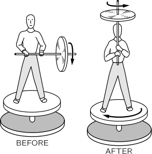
Rotations
The center of mass
Let us say M is the sum of all the masses, i.e., the total mass. Then if we define a certain vector R to be 
then the external force is the total mass times the acceleration of an imaginary point whose location is R. This point is called the center of mass of the body. It is a point somewhere in the "middle" of the object, a kind of average r in which the different r/s have weights or importances proportional to the masses.
Rotation of a rigid body
We have a velocity of turning, ω=dθ/dt, which tells us how much the angle changes in a second, just as v=ds/dt describes how fast a thing moves, or how far it moves in a second.
The change in the x and y directions is simply the projection of rΔθ in the x,y-directions:
Δx= −y Δθ Δy=+x Δθ
If the object is turning with a given angular velocity ω, we find, by dividing both sides by Δt, that the velocity of the particle is
![[ v_x=−omega , y quad v_y=omega , x quad Rightarrow quad {bf v}=omegatimes {bf r} ]](http://tlonworld.com/wp-content/ql-cache/quicklatex.com-e01632c12121578e46bffbe4d567018b_l3.svg "Rendered by QuickLaTeX.com")
Angular momentum
The work done to turn the object through a very small angle is
![[ Delta W=F_x, Delta x+F_y , Delta y = (x, F_y-y, F_x), Deltatheta ]](http://tlonworld.com/wp-content/ql-cache/quicklatex.com-157da37697a8d73a9163a1300253ec85_l3.svg "Rendered by QuickLaTeX.com")
This “strange combination” :  is what we call the torque.
The angular momentum is defined as
![[ L= m( x { dyover dt} -y {dxover dt} )=x p_y- y p_x ]](http://tlonworld.com/wp-content/ql-cache/quicklatex.com-23a3320a1bfc9f459b4152fa8fcf8804_l3.svg "Rendered by QuickLaTeX.com")
The rate of change of the total angular momentum about any axis is equal to the external torque about that axis:
![[ tau = { dLover dt} ]](http://tlonworld.com/wp-content/ql-cache/quicklatex.com-6c6c13fc1e4c37ecb6d4bf21430bd854_l3.svg "Rendered by QuickLaTeX.com")
Although our present discussion is nonrelativistic, the second form for L given above is relativistically correct. In absence of torque
angular momentum is conserved. The law of conservation of angular momentum may be demonstrated with a rapidly spinning wheel, or gyroscope, as follows (see Figure). If we sit on a swivel chair and hold the spinning wheel with its axis horizontal, the wheel has an angular momentum about the horizontal axis. Angular momentum around a vertical axis cannot change because of the (friction- less) pivot of the chair, so if we turn the axis of the wheel into the vertical, then the wheel would have angular momentum about the vertical axis, because it is now spinning about this axis. But the system (wheel, ourself, and chair) cannot have a vertical component, so we and the chair have to turn in the direction opposite to the spin of the wheel, to balance it.
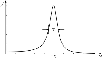
The harmonic oscillator and resonance
The harmonic oscillator
There are several mechanical systems whose motion is determined by differential equations with constant coefficients: the oscillations of a mass on a spring; the oscillations of charge flowing back and forth in an electrical circuit; the vibrations of a tuning fork which is generating sound waves; the analogous vibrations of the electrons in an atom, which generate light waves; the equations for the operation of a servosystem, such as a thermostat trying to adjust a temperature; complicated interactions in chemical reactions; the growth of a colony of bacteria in interaction with the food supply and the poisons the bacteria produce; foxes eating rabbits eating grass, and so on.
The harmonic oscillator is the simplest example of a mechanical system whose motion follows a linear differential equation with constant coefficients
![[ m {d^2xover dt}=-k x quad Rightarrow quad x =A, cos(w_0 t)+B, sin (w_0 t) ]](http://tlonworld.com/wp-content/ql-cache/quicklatex.com-861fc73631d0e534566b4612df108782_l3.svg "Rendered by QuickLaTeX.com")
with A,B constants and  . In presence of an external driving force :
![[ m { d^2x over dt^2}=-k x+F(t) ]](http://tlonworld.com/wp-content/ql-cache/quicklatex.com-a35205ed639f46b4d2b11d45ff74a23e_l3.svg "Rendered by QuickLaTeX.com")
For example for a force F=F0 cos( w t), the solution requires: B=0,  !!
!!
Resonance
Let us add a friction term. Ordinarily such a problem is very difficult because of the character and complexity of the frictional term. There are, however, many circumstances in which the frictional force is proportional to the speed with which the object moves. An example of such friction is the friction for slow motion of an object in oil or a thick liquid. There is no force when it is just standing still, but the faster it moves the faster the oil has to go past the object, and the greater is the resistance. So we we consider the equation of motion
![[ m {d^2x over dt^2} + c ,{dxover dt}+k x=F(t)=F_0, cos( omega t+Delta) ]](http://tlonworld.com/wp-content/ql-cache/quicklatex.com-10c0c1b977963a36028b75ac92823f2a_l3.svg "Rendered by QuickLaTeX.com")
We can think of x as F as the real part of x, F defined as
![[ x=rho, F_0 e^{iomegat+iDelta +itheta} quadquad F= F_0 , e^{iomega, t+iDelta } ]](http://tlonworld.com/wp-content/ql-cache/quicklatex.com-3fade881d76e48ed1f3ced483bce0ae4_l3.svg "Rendered by QuickLaTeX.com")
with
![[ rho^2={ 1over m^2left[ (omega^2−omega_0^2)^2+gamma^2 omega^2right]} quad tantheta=−{gamma omega over omega_0^2−omega^2} ]](http://tlonworld.com/wp-content/ql-cache/quicklatex.com-95a3691afc4379ce8a73dfe0875504b7_l3.svg "Rendered by QuickLaTeX.com")
This tells us that the amplitude of the response is the magnitude of the force F multiplied by a certain magnification factor, ρ; this gives us the “amount” of oscillation. This magnification is maximum at w=w0, we says that the system has a resonance at w=w0.
It also tells us, however, that x is not oscillating in phase with the force, which has the phase Δ, but is shifted by an extra amount θ. Therefore ρ and θ represent the size of the response and the phase shift of the response.
If we call the maximum height of the curve of  one unit, and we ask for the width of the curve, at one half the maximum height, the full width at half the maximum height of the curve is γ, supposing that γ is small. The resonance is sharper and sharper as the frictional effects are made smaller and smaller.
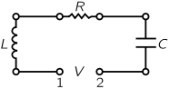
Electrical resonance
The simplest and broadest technical applications of resonance are in electricity. In the electrical world there are a number of objects which can be connected to make electric circuits. The three main kinds of circuit elements are the following:
1) The first is called a capacitor; an example is two plane metallic plates spaced a very small distance apart by an insulating material. The potential difference across a capacitor is proportional to the charge: V=q/C, where C is the capacitance of the object 2) The second kind of circuit element is called a resistor; it offers resistance to the flow of electrical current. It turns out that metallic wires and many other substances resist the flow of electricity in this manner: if there is a voltage difference across a piece of some substance, there exists an electric current I = dq/dt that is proportional to the electric voltage difference: V = R I = R dq/dt. The proportionality coefficient is called the resistance R. This relationship may already be familiar to you; it is Ohm's law.
3) The third element is the coil which builds up a magnetic field within itself when there is a current in it. A changing magnetic field develops in the coil a voltage that is proportional to  .
.
Suppose we make a circuit in which we have connected the three circuit elements in series (see figure). The voltage across the whole thing
is
![[ L {d^2qover dt^2} +R { dqover dt}+{qover C}=V(t) ]](http://tlonworld.com/wp-content/ql-cache/quicklatex.com-a62a0c4483ac8b0b1e22cde89525b33c_l3.svg "Rendered by QuickLaTeX.com")
This is the same equation of the forced harmonic oscillator with friction with  , γ=(R/L).
Resonance in nature
There are many circumstances in nature in which something is "oscillating" and in which the resonance phenomenon occurs.
The first on a large scale: the atmosphere of the whole earth. If the atmosphere, which we suppose surrounds the earth evenly on all sides, is pulled to one side by the moon or, rather, squashed prolate into a double tide, and if we could then let it go, it would go sloshing up and down; it is an oscillator. This oscillator is driven by the moon, which is effectively re- volving about the earth; any one component of the force, say in the x-direction, has a cosine component, and so the response of the earth's atmosphere to the tidal pull of the moon is that of an oscillator. One might think that we only have one point on this resonance curve, since we only have the one frequency, corresponding to the rotation of the earth under the moon, which occurs at a period of 12.42, but from the size of the atmospheric tides, and from the phase, the amount of delay, we can get both ρ and θ. If someone disturbed the atmosphere, it would oscillate with the frequency w0. Now there was such a sharp disturbance in 1883; the Krakatoa volcano exploded and half the island blew off, and it made such a terrific explosion in the atmosphere that the period of oscillation of the atmosphere could be measured. It came out to 10 hours and 20 minutes.
Next we consider a sodium chloride crystal, which has sodium ions and chlorine ions next to each other. These ions are electrically charged, alternately plus and minus. Now there is an interesting oscillation possible. Suppose that we could drive all the plus charges to the right and all the negative charges to the left, and let go; they would then oscillate back and forth, the sodium lattice against the chlorine lattice. If we apply an electric field on the crystal, it will push the plus charge one way and the minus charge the other way! So, by having an external electric field we can perhaps get the crystal to oscillate. The frequency of the electric field needed is so high, however, that it corresponds to infrared radiation! So we try to find a resonance curve by measuring the absorption of infrared light by sodium chloride.
Next we consider the swinging of a magnet. If we have a magnet, with north and south poles, in a constant magnetic field, the N end of the magnet will be pulled one way and the S end the other way, and there will in general be a torque on it, so it will vibrate about its equilibrium position, like a compass needle. However, the magnets we are talking about are atoms. These atoms have an angular momentum, the torque does not produce a simple motion in the direction of the field, but instead, of course, a precession. Now we can disturb or drive the swinging and measure an absorption.
If we bombard a lithium atom with protons we discover that a certain reaction, producing γ-rays, actually has a very sharp maximum typical of resonance. The reason is that in quantum mechanics what we think of classically as the energy will turn out to be really related to a frequency of a wave amplitude.
A resonance is found in a certain reaction among strange particles, a reaction in which a K− and a proton interact. The resonance is detected by seeing how many of some kinds of particles come out, and depending on what and how many come out, one gets different curves, but of the same shape and with the peak at the same energy. We thus determine that there is a resonance at a certain energy for the K− meson. That presumably means that there is some kind of a state, or condition, corresponding to this resonance, which can be attained by putting together a K− and a proton. This is a new particle, or resonance.
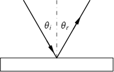
Optics: the principle of least time
Light
Reflection and refraction
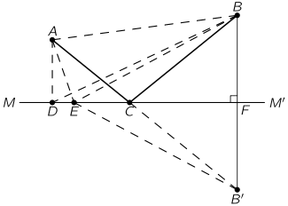
Fermat principle of least time
In the further development of science, we want more than just a formula. First we have an observation, then we have numbers that we measure, then we have a law which summarizes all the numbers. But the real glory of science is that we can find a way of thinking such that the law is evident. The first way of thinking that made the law about the behavior oflight evident was discovered by Fermat in about 1650, and it is called the principle ofleast time, or Fermat's principle. His idea is this: that out of all possible paths that it might take to get from one point to another, light takes the path which requires the shortest time.
More precisely the light takes a path such that there are many other paths nearby which take almost exactly the same time.
Two points, A and B, and a plane mirror, MM'. What is the way to get from A to Bin the shortest time? The answer is to go straight from A to B! But if we add the extra rule that the light has to strike the mirror. We construct on the other side of MM' an artificial point B'. The shortest line is that going through point C as a straight line from A to B'! In other words, we have to find the point where we go toward the artificial point.
Originally, the statement was made by Hero of Alexandria that the light travels in such a way that it goes to the mirror and to the other point in the shortest possible distance, so it is not a modern theory. It was this that inspired Fermat to suggest to himself that perhaps refraction operated on a similar basis. But for refraction, light obviously does not use the path of shortest distance, so Fermat tried the idea that it takes the shortest time.
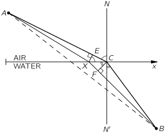
In the left figure, our problem is again to go from A to B in the shortest time. We are at point A on land, and we see the accident, and we can run and can also swim. But we can run faster than we can swim. What do we do? Do we go in a straight line? (Yes, no doubt!) However, by using a little more intelligence we would realize that it would be advan- tageous to travel a little greater distance on land in order to decrease the distance in the water, because we go so much slower in the water. At any rate, let us try to show that the final solution to the problem is the path ACB, and that this path takes the shortest time of all possible ones. This means that if we move the point X to points near C, in the first approximation there is essentially no change in time. But supposing that in the water the speed is 1/n times as fast as in air, then we must have EC = n· XF or equivalently XC sin EXC = n · XC sin XCF resulting into sin θi=n sin θr
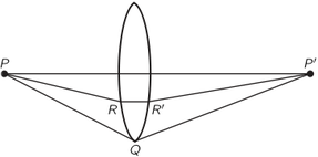
Applications of the Fermat principle
When we see the sun setting, it is already below the horizon! The earth's atmosphere is thin at the top and dense at the bottom. Light travels more slowly in air than it does in a vacuum, and so the light of the sun can get to point S beyond the horizon more quickly if, instead of just going in a straight line, it avoids the dense regions where it goes slowly by getting through them at a steeper tilt. When it appears to go below the horizon, it is actually already well below the horizon.
Another example of this phenomenon is the mirage that one often sees while driving on hot roads. One sees "water" on the road, but when he gets there, it is as dry as the desert! The phenomenon is the following. What we are really seeing is the sky light "reflected" on the road: The air is very hot just above the road but it is cooler up higher. Hotter air is more expanded than cooler air so the light goes faster in the hot region than in the cool region. Therefore, instead of the light deciding to come in the straightforward way, it also has a least-time path by which it goes into the region where it goes faster for awhile, in order to save time.
Suppose that we had a piece of glass in which light goes slower than it does in the air (Fig. left). Now consider a ray which goes in air
in the path PQP'. That is a longer path than from P directly to P' and no doubt takes a longer time. But if we were to insert a piece of glass of just the right thickness (we shall later figure out how thick) it might exactly compensate the excess time that it would take the light to go at an angle! In those circumstances we can arrange that the time the light takes to go straight through is the same as the time it takes to go in the path PQP'.
With this shape, all the light which comes from P will go to P'. This, of course, is well known to us, and we call such a device a converging lens.
A more precise statement of the Fermat principle
The light does not seem to be in the form of waves at all. Instead the rays seem to be made up of photons, and they actually produce clicks in a photon counter, if we are using one. The brightness of the light is proportional to the average number of photons that come in per second, and what we calculate is the chance that a photon gets from A to B, say by hitting the mirror. The law for that chance is the following very strange one. Take any path and find the time for that path; then make a complex number, or draw a little complex vector, ρ e^iθ, whose angle θ is proportional to the time. The number of turns per second is the frequency of the light. Now take another path; it has, for instance, a different time, so the vector for it is turned through a different angle—the angle being always proportional to the time. Take all the available paths and add on a little vector for each one; then the answer is that the chance of arrival of the photon is proportional to the square of the length of the final vector, from the beginning to the end! Now let us show how this implies the principle of least time for a mirror. We consider all rays, all possible paths ADB, AEB, ACB, etc., in the Figure above. The path ADB makes a certain small contribution, but the next path, AEB, takes a quite different time, so its angle θ is quite different. Let us say that point C corresponds to minimum time, where if we change the paths the times do not change. So for awhile the times do change, and then they begin to change less and less as we get near point C. So the arrows which we have to add are coming almost exactly at the same angle for awhile near C, and then gradually the time begins to increase again, and the phases go around the other way, and so on. Eventually, we have quite a tight knot. The total probability is the distance from one end to the other, squared. Almost all of that accumulated probability occurs in the region where all the arrows are in the same direction (or in the same phase). All the contributions from the paths which have very different times as we change the path, cancel themselves out by pointing in different directions.
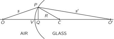
Geometrical optics
The focal length of a spherical surface
Suppose that we have a point at 0, at a distances from the front surface ofthe glass, and another point 0' at a distance s' inside the glass, and we desire to arrange the curved surface in such a manner that every ray from 0 which hits the surface, at any point P, will be bent so as to proceed toward the point 0'. For that to be true, we have to shape the surface in such a way that the time it takes for the light to go from 0 to P, that is, the distance OP divided by the speed of light (the speed here is unity), plus n · O'P, which is the time it takes to go from P to 0', is equal to a constant independent of the point P. This condition supplies us with an equation for determining the surface. The answer is that the surface is a very complicated fourth-degree curve, and the student may entertain himself by trying to calculate it by analytic geometry. It is simpler to try a special case that corresponds to s→∞, because then the curve is a second-degree curve and is more recognizable.
Supposing P is close to the axis, we drop a perpendicular PQ such that the height PQ is h. For a moment, we imagine that the surface is a plane passing through P. In that case, the time needed to go from O to P would exceed the time from O to Q, and also, the time from P to O′ would exceed the time from Q to O′. But that is why the glass must be curved, because the total excess time must be compensated by the delay in passing from V to Q. Now the excess time along route OP is h^2/2s, and the excess time on the other route is n h^2/2s′. This excess time, which must be matched by the delay in going along VQ, differs from what it would have been in a vacuum, because there is a medium present. Therefore we discover that the law that connects the distances s and s′, and that gives us the radius of curvature R of the surface that we need, is
![[ {1over s}+{n over s′}={n-1over R}={1over f} ]](http://tlonworld.com/wp-content/ql-cache/quicklatex.com-466e25fd5a17ba98a984e50efbdcc843_l3.svg "Rendered by QuickLaTeX.com")
A given lens will (so long as we limit ourselves to paraxial rays) focus not only from 0 to 0', but between an infinite number of other pairs of points, so long as those pairs of points bear the relationship that I/s + n/s' is a constant, characteristic of the lens. Now consider the interesting case where R is equal to infinity; then we have 1/s + n/s' = 0. In other words, s' = -ns, which means that if we look from a dense medium into a rare medium and see a point in the rare medium, it appears to be deeper by a factor n. When we look at the bottom of a swimming pool from above, it does not look as deep as it really is, by a factor 3/4, which is the reciprocal of the index of refraction of water.
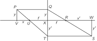
Magnification
When we set up a lens so as to focus light from a small filament onto a "point'' on a screen, we notice that on the screen we get a "picture" of the same filament, except of a larger or smaller size than the true filament.
(1) Any ray that comes in parallel on one side proceeds toward a certain par- ticular point called the focus on the other side, at a distance/from the lens.
(2) Any ray that arrives at the lens from the focus on one side comes out parallel to the axis on the other side. One finds te lens formula:y′/y=x′/f=f/xAberrationLight of different colors has different speeds, or different indices of refraction, in the glass, and therefore the focal length of a given lens is different for different colors. So if we image a white spot, the image will have colors, because when we focus for the red, the blue is out of focus, or vice versa. This property is called chromatic aberration.
Resolving power
Electromagnetic radiation
Electromagnetism
It seems a miracle that someone talking in Europe can, with mere electrical influences, be heard thousands of miles away in Los Angeles. How is it possible? It is because the fields do not vary as the inverse square, but only inversely as the first power of the distance. The laws of electricity and magnetism, as known at the end of the 19th century, are these: the electrical forces acting on a charge q can be described by two fields, called E and B, and the velocity v of the charge q, by the equation F=q(E+v×B). To complete this law, we have to say what the formulas for E and B are in a given circumstance: if a number of charges are present, E and the B are each the sum of contributions, one from each individual charge. So if we can find the E and B produced by a single charge, we need only to add all the effects from all the charges in the universe to get the total E and B! This is the principle of superposition.The electric field, E, is given by
![[ {bf E}=-{qover 4pi epsilon_0 } left[ {{bf e}_{r}over r^2} +{rover c}{ dover dt} left({ {bf e}_rover r^2}right)+{1over c^2} {d^2over dt^2} {bf e}_r right] label{eradiation} ]](http://tlonworld.com/wp-content/ql-cache/quicklatex.com-025f55e3b7f3dc39f65aee5a844fae02_l3.svg "Rendered by QuickLaTeX.com")
What do the various terms tell us? Take the first term,  . That, of course, is Coulomb’s law, which we already know: q is the charge that is producing the field;
  is the unit vector in the direction from the point P where E is measured, r is the distance from P to q. But, Coulomb’s law is wrong. The discoveries of the 19th century showed that influences cannot travel faster than a certain fundamental speed c, which we now call the speed of light. It is not correct that the first term is Coulomb’s law, not only because it is not possible to know where the charge is now and at what distance it is now, but also because the only thing that can affect the field at a given place and time is the behavior of the charges in the past. How far in the past? The time delay, or retarded time, so-called, is the time it takes, at speed c, to get from the charge to the field point P. The delay is r/c. So to allow for this time delay, we put a little prime on r, meaning how far away it was when the information now arriving at P left q. The next term calculate the delayed coulomb field and add a correction to it, which is its rate of change times the time delay that we use. There is a third term-the second derivative, with respect to t, of the unit vector in the direction of the charge.
The magnetic field is given by
![[ {bf B}= -{{bf e}_r times E over c} ]](http://tlonworld.com/wp-content/ql-cache/quicklatex.com-cce4e66e0a4a96470622872a078d922a_l3.svg "Rendered by QuickLaTeX.com")
Radiation
Of the terms appearing in E, the first one evidently goes inversely as the square of the distance, and the second is only a correction for delay, so it is easy to show that both of them vary inversely as the square of the distance. All of the effects we are interested in come from the third term, which is not very complicated, after all. What this term says is: look at the charge and note the direction of the unit vector (we can project the end of it onto the surface of a unit sphere). As the charge moves around, the unit vector wiggles, and the acceleration of that unit vector is what we are looking for. Thus
![[ {bf E}=−{qover 4pi epsilon_0 c^2 } {d^2over dt^2} {bf e}_r ]](http://tlonworld.com/wp-content/ql-cache/quicklatex.com-5ca66981f85d445f69dd1d8724102131_l3.svg "Rendered by QuickLaTeX.com")
is a statement of the laws of radiation, because that is the only important term when we get far enough away that the fields are varying inversely as the distance.
If the charged object is moving in a very small motion and it is laterally displaced by the distance x(t), then the angle that the unit vector er' is displaced is x/r, and since r is practically constant, the x-component of  is simply the acceleration of x itself at an earlier time, and so finally we get the law we want, which is
![[ E_x(t)=-{qover 4pi epsilon_0 c^2, r} , a_x(t-r,c) ]](http://tlonworld.com/wp-content/ql-cache/quicklatex.com-6dbca3c5b22ca9231770400497dd51f4_l3.svg "Rendered by QuickLaTeX.com")
Only the component of ax perpendicular to the line of sight is important.
Dipole radiators
Consider the combine effects of two oscillators at a given point. Let us take the simple case, where the oscillators are situated with their centers in the same horizontal plane as the detector, and the line of vibration is vertical. In particular consider two such oscillators at half a wavelength apart in a N-S direction, oscillating together in the same phase, which we call zero phase. Now we would like to know the intensity of the radiation in various directions. By the intensity we mean the amount of energy that the field carries past us per second, which is proportional to the square of the field, averaged in time. So the thing to look at, when we want to know how bright the light is, is the square of the electric field, not the electric field itself. In the W direction the intensity is now zero, because one oscillator is "pushing" when the other one is "pulling." But in the N direction the signal from the near one comes at a certain time, and that of the other comes half a period later. But the latter was originally half a period behind in timing, and therefore it is now exactly in time with the first one, and so the intensity in this direction is maximal.
if we build an antenna system and want to send a radio signal, say, to Hawaii, we set the antennas up as above and we broadcast with our two antennas in phase, because Hawaii is to the west of us. Then we decide that tomorrow we are going to broadcast toward Alberta, Canada. Since that is north, not west, all we have to do is to reverse the phase of one of our antennas, and we can broadcast to the north. So we can build antenna systems with various arrangements.
The difraction gratin
Suppose that we had a lot of parallel wires, equally spaced at a spacing d, and a radiofrequency source very far away, practically at infinity, which is generat- ing an electric field which arrives at each one of the wires at the same phase (it is so far away that the time delay is the same for all of the wires). (One can work out cases with curved arrays, but let us take a plane one.) Then the external electric field will drive the electrons up and down in each wire. That is, the field which is coming from the original source will shake the electroiJ.s up and down, and in moving, these represent new generators. This phenomenon is called scattering: a light wave from some source can induce a motion of the electrons in a piece of material, and these motions generate their own waves.
Interference
Sinusoidal waves
We can define a quantity called the wave number, symbolized as k. This is defined as the rate of change of phase with distance (radians per meter).
The wavelength is the distance occupied by one complete cycle. It is easy to see, then, that the wavelength is  .
.
Two dipole radiators
In combining the effects of two oscillators to find the net field at a given point. This is very easy in the few cases that we considered in the previous chapter. We shall first describe the effects qualitatively, and then more quantitatively. Let us take the simple case, where the oscillators are situated with their centers in the same horizontal plane as the detector, and the line of vibration is vertical.
We would like to know the intensity of the radiation in various directions. By the intensity we mean the amount of energy that the field carries past us per second, which is proportional to the square of the field, averaged in time. So the thing to look at, when we want to know how bright the light is, is the square of the electric field, not the electric field itself.
Suppose the oscillators are again one-half a wavelength apart, but the phase a of one is set half a period behind the other in its oscillation. In the W direction the intensity is now zero, because one oscillator is "pushing" when the other one is "pulling." But in the N direction the signal from the near one comes at a certain time, and that of the other comes half a period later. But the latter was originally half a period behind in timing, and therefore it is now exactly in time with the first one, and so the intensity in this direction is 4 units.
if we build an antenna system and want to send a radio signal, say, to Hawaii, we set the antennas up and we broadcast with our two antennas in phase, because Hawaii is to the west of us. Then we decide that tomorrow we are going to broadcast toward Alberta, Canada. Since that is north, not west, all we have to do is to reverse the phase of one of our antennas, and we can broadcast to the north. So we can build antenna systems with various arrangements.
Diffraction
The diffraction gratin
Suppose that we had a lot of parallel wires, equally spaced at a spacing d, and a radiofrequency source very far away, practically at infinity, which is generat- ing an electric field which arrives at each one of the wires at the same phase.
Then the external electric field will drive the electrons up and down in each wire. That is, the field which is coming from the original source will shake the electroiJ.s up and down, and in moving, these represent new generators. This phenomenon is called scattering: a light wave from some source can induce a motion of the electrons in a piece of material, and these motions generate their own waves.
A diffraction grating consists of nothing but a plane glass sheet, transparent and colorless, with scratches on it. There are often several hundred scratches to the millimeter, very carefully arranged so as to be equally spaced. The effect of such a grating can be seen by arranging a projector so as to throw a narrow, vertical line of light (the image of a slit) onto a screen. When we put the grating into the beam, with its scratches vertical, we see that the line is still there but, in addition, on each side we have another strong patch of light which is colored. This, of course, is the slit image spread out over a wide angular range, because the angle Bin (30.6) depends upon X, and lights of different colors, as we know, correspond to different frequencies, and therefore different wavelengths. The longest visible wavelength is red, and since d sin B = X, that requires a larger B. And we do, in fact, find that red is at a greater angle out from the central image!
We begin to understand the basic machinery of reflection: the light that comes in generates motions of the atoms in the reflector, and the reflector then regenerates a new wave, and one of the solutions for the direction of scattering, the only solution if the spacing of the scatterers is small compared with one wavelength, is that the angle at which the light comes out is equal to the angle at which it comes in!
Resolving power of a gratin
Supposing that there were two sources of slightly different frequency, or slightly different wavelength, how close together in wavelength could they be such that the grating would be unable to tell that there were really two different wavelengths there?
Rayleigh's criterion: Two frequency are resolved when the first minimum from one bump sit at the maximum of the other.
The ratio  is called the resolving power of a grating;
The parabolic anthena
Now suppose that the radio source is at a slight angle 0 from the vertical. Then the various antennas are receiving signals a little out of phase. The receiver adds all these out-of-phase signals together, and so we get nothing, if the angle  is too big.
The smallest angle that can be resolved by an antenna array of length L is  .
.
Colored films crystals
if we look at the reflection of a light source in a thin film, we see the sum of two waves; if the thicknesses are small enough, these two waves will produce an inter- ference, either constructive or destructive, depending on the signs of the phases. It might be, for instance, that for red light, we get an enhanced reflection, but for blue light, which has a different wavelength, perhaps we get a destructively inter- fering reflection, so that we see a bright red reflection. If we change the thickness, i.e., if we look at another place where the film is thicker, it may be reversed, the red interfering and the blue not, so it is bright blue, or green, or yellow, or whatnot. So we see colors when we look at thin films and the colors change if we look at different angles, because we can appreciate that the timings are different at different angles.
We used a grating and we saw the diffracted image on the screen. If we had used monochromatic light, it would have been at a certain specific place. Then there were various higher-order images also. From the positions of the images, we could tell how far apart the lines on the grating were, if we knew the wavelength of the light.
This principle is used to dis· cover the positions of the atoms in a crystal. The only complication is that a crystal is three-dimensional; it is a repeating three-dimensional array of atoms. We cannot use ordinary light, because we must use something whose wavelength is less than the space between the atoms or we get no effect; so we must use radiation of very short wavelength, i.e., x-rays. So, by shining x-rays into a crystal and by noticing how intense is the reflection in the various orders, we can determine the arrangement of the atoms inside without ever being able to see them with the eye!
The origin of the refractive index
The index of diffraction
It is approximately true that light or any electrical wave does appear to travel at the speed cjn through a material whose index of refraction is n, but the fields are still produced by the motions of all the charges-including the charges moving in the material-and with these basic contributions of the field travelling at the ultimate velocity c.
We shall try to understand the effect in a very simple case. A source which we shall call "the external source" is placed a large distance away from a thin plate of transparent material, say glass. We inquire about the field at a large distance on the opposite side of the plate.
According to the principles we have stated earlier, an electric field anywhere that is far from all moving charges is the (vector) sum of the fields produced by the external source (at S) and the fields produced by each of the charges in the plate of glass, every one with its proper retardation at the velocity c.
When the electric field ofthe source acts on these atoms it drives the electrons up and down, because it exerts a force on the electrons. And moving electrons generate a field-they constitute new radiators. These new radiators are related to the source S, because they are driven by the field of the source. The total field is not just the field of the source S, but it is modified by the additional contribution from the other moving charges.
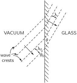 Before we proceed with our study of how the index of refraction comes about, we should understand that all that is required to understand refraction is to under- stand why the apparent wave velocity is different in different materials. The bending of light rays comes about just because the effective speed of the waves is different in the materials. To remind you how that comes about we have drawn in the left figure several successive crests of an electric wave which arrives from a vacuum onto the surface of a block of glass. The arrow perpendicular to the wave crests indicates the direction of travel of the wave. Now all oscillations in the wave must have the same frequency. (We have seen that driven oscillations have the same frequency as the driving source.) This means, also, that the wave crests for the waves on both sides of the surface must have the same spacing along !he surface because they must travel together, so that a charge sitting at the boundary will feel only one frequency. The shortest distance between crests of the wave, however, is the wavelength which is the velocity divided by the frequency. On the vacuum side it is
  and on the other side it is
  or
or  , if
, if  is the velocity of the wave. From the figure we can see that the only way for the waves to “fit” properly at the boundary is for the waves in the material to be travelling at a different angle with respect to the surface. From the geometry of the figure you can see that for a “fit” we must have
  or
or  , which is Snell’s law.
The index of refraction is given by
![[ n=1+{ N, q_e^2 over 2epsilon_0, m (w_0^2-w^2)} ]](http://tlonworld.com/wp-content/ql-cache/quicklatex.com-08cab1981e059fbddf149d2b65c6c249_l3.svg "Rendered by QuickLaTeX.com")
with  the number of atoms per unit volume of the plate,
  ,
,  the charge and mass of an electron, w the angular frequency of the radiation,
  the resonant frequency of an electron bound in the atom.
Dispersion
For most ordinary gases (for instance, for air, most colorless gases, hydrogen, helium, and so on) the natural frequencies of the electron oscillators correspond to ultraviolet light. These frequencies are higher than the frequencies of visible light, that is, w0 is much larger than w of visible light, and to a first approximation, we can disregard w2 in comparison with Then we find that the index is nearly constant. So for a gas, the index is nearly constant. This is also true for most other transparent substances, like glass. If we look at our expression a little more closely, however, we notice that as w rises, taking a little bit more away from the denominator, the index also rises. So n rises slowly with frequency. The index is higher for blue light than for red light. That is the reason why a prism bends the light more in the blue than in the red.
The phenomenon that the index depends upon the frequency is called the phenomenon of dispersion, because it is the basis of the fact that light is "dispersed" by a prism into a spectrum.
At frequencies very close to the natural frequency the index can get enor- mously large, because the denominator can go to zero.
If we beam x-rays on matter, or radiowaves (or any electric waves) on free electrons the term  becomes negative, and we obtain the result that n is less than one. That means that the effective speed of the waves in the substance is faster than c! Can that be correct?
It is correct. In spite of the fact that it is said that you cannot send signals any faster than the speed of light, it is nevertheless true that the index of refraction of materials at a particular frequency can be either greater or less than I.
What the index tell us is the speed at which the nodes (or crests) of the wave travel. The node of a wave is not a signal by itself. In a perfect wave, which has no modulations of any kind, i.e., which is a steady oscillation, you cannot really say when it "starts," so you cannot use it for a timing signal. In order to send a signal you have to change the wave somehow, make a notch in it, make it a little bit fatter or thinner.
We should remark that our analysis of the refractive index gives a result that is somewhat simpler than you would actually find in nature. To be completely accurate we must add some refinements. First, we should expect that our model of the atomic oscillator should have some damping force (otherwise once started it would oscillate forever, and we do not expect that to happen). In presence of a damping with coefficient  we replace in the denominator of the refractive index formula by
  .
.
Absortion
As the wave goes through the material, it is weakened. The material is "absorbing" part of the wave. The wave comes out the other side with less energy. We should not be surprised at this, because the damping we put in for the oscillators is indeed a friction force and must be expected to cause a loss of energy. We see that the imaginary part of a complex index of refraction n represents an absorption (or "attenuation") of the wave.
For instance as in glass, the absorption of light is very small. This is to be expected from our Eq. (31.20), because the imaginary part of the denominator,  , is much smaller than the term . But if the light fre- quency w is very close to then the index becomes almost completely imaginary. The absorption of the light becomes the dominant effect. It is just this effect that gives the dark lines in the spectrum of light which we receive from the sun. The light from the solar surface has passed through the sun's atmosphere (as well as the earth's), and the light has been strongly absorbed at the resonant frequencies of the atoms in the solar atmosphere.
The observation of such spectral lines in the sunlight allows us to tell the resonant frequencies of the atoms and hence the chemical composition of the sun's atmosphere. The same kind of observations tell us about the materials in the stars. From such measurements we know that the chemical elements in the sun and in the stars are the same as those we find on the earth.
Polarization
The electric vector of light
In ideally monochromatic light, the electric field must oscillate at a definite frequency, but since the x-component and the yy-component can oscillate independently at a definite frequency, we must first consider the resultant effect produced by superposing two independent oscillations at right angles to each other. When the x-vibration and the y-vibration are not in phase, the electric field vector moves around in an ellipse. The motion in a straight line is a particular case corresponding to a phase difference of zero (or an integral multiple of  ); motion in a circle corresponds to equal amplitudes with a phase difference of 90 degrees (or any odd integral multiple of
  ).
).
Light is linearly polarized (sometimes called plane polarized) when the electric field oscillates on a straight line.
Relativistic effects of radiation
Moving sources
We recall that the fundamental laws of electrodynamics say that, at large distances from a moving charge, the electric field is given by the formula
![[ {bf E}=-{qover 4pi epsilon_0 c^2} {d^2 {bf e}_{R'}over dt^2 } ]](http://tlonworld.com/wp-content/ql-cache/quicklatex.com-631bb75136c84d8f30150c69b677ae8a_l3.svg "Rendered by QuickLaTeX.com")
The second derivative of the unit vector  which points in the apparent direction of the charge, is the determining feature of the electric field.
Associated with the electric field is a magnetic field, always at right angles to the electric field and at right angles to the apparent direction of the source, given by the formula
![[ B=- {bf e}_{R'}times {bf E}/c ]](http://tlonworld.com/wp-content/ql-cache/quicklatex.com-814522176e121b45a88c5552bec62cb6_l3.svg "Rendered by QuickLaTeX.com")
Let the coordinates of the charge be (x,y,z) with z measured along the direction of observation. Now the direction of the vector depends mainly on x and y, but hardly at all upon z. The transverse components of the unit vector are x/R and y/R with R the distance from the source. One finds

If the time of observation is called t then the time τ to which this corresponds is delayed by the total distance that the light has to go, divided by the speed of light. In the first approximation, this delay is R/c but in the next approximation we must include the effects of the position in the z-direction at the time τ. Thus τ is determined by
![[ t=tau+R, c+z(tau) quadquad x'(t)=x(tau) ]](http://tlonworld.com/wp-content/ql-cache/quicklatex.com-037c91a4b6dc562b188e11d799838488_l3.svg "Rendered by QuickLaTeX.com")
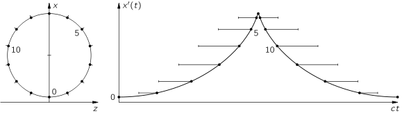
 for a source moving on a circle in the (x,z) plane. For a source moving fast the cusp gets very sharp.
In the synchrotron we have electrons which go around in circles in a uniform magnetic field.; they are travelling at very nearly the speed c, and it is possible to see the above radiation as actual light! First, let us see why they go in circles. We know that the force on a particle in a magnetic field is given by
![[ {bf F}=q , {bf v} times {bf B} ]](http://tlonworld.com/wp-content/ql-cache/quicklatex.com-f38e53940e960ad3a5ef01e85b11ab33_l3.svg "Rendered by QuickLaTeX.com")
and it is at right angles both to the field and to the velocity. As usual, the force is equal to the rate of change of momentum with time. Since the force is at right angles to the velocity, the kinetic energy, and therefore the speed, remains constant. All the magnetic field does is to change the direction of motion. In a short time  , the momentum vector changes at right angles to itself by an amount
  and therefore p turns through an angle
  . But in this same time the particle has gone a distance Δs=vΔt =RΔθ. Combining this with the previous expressions, we find that the particle must be moving in a circle of radius R, with momentum
![[ p=q , B , R ]](http://tlonworld.com/wp-content/ql-cache/quicklatex.com-0713100d7e7201527a5588930db43792_l3.svg "Rendered by QuickLaTeX.com")
![[ omega ={vover R}= {q, v, Bover p} ]](http://tlonworld.com/wp-content/ql-cache/quicklatex.com-0b1167dfaed6f390039d10ad588bb4c8_l3.svg "Rendered by QuickLaTeX.com")
If q is expressed in terms of the electronic charge the kinetic energy pc can be measured in units of the electron volt
![[ pc (eV)=3times 10^8 {qover q_e} , B, R ]](http://tlonworld.com/wp-content/ql-cache/quicklatex.com-5b84186d22594102ca216ce05562d20d_l3.svg "Rendered by QuickLaTeX.com")
The mks unit of magnetic field is called a weber per square meter. Today, electromagnets wound with superconducting wire are able to produce steady fields of over 10 mks units. The field of the earth is weber per meter square at the equator.
We could imagine the synchrotron running at a billion electron volts, then, if we had a B corresponding to, say, 1 kms then we see that R would have to be 3.3 meters. The actual radius of the Caltech synchrotron is 3.7 meters, the field is a little bigger, and the energy is 1.5 billion, but it is the same idea.
We know that the total energy, including the rest energy, is given by  and for an electron the rest energy corresponding to
  , so when
  we can neglect the rest energy. If
  , it is easy to show that the speed differs from the speed of light by but one part in eight million!
We turn now to the radiation emitted by such a particle. A particle moving on a circle of radius 3.3 meters, or 20 meters circumference, goes around once in roughly the time it takes light to go 20 meters. So the wavelength that should be emitted by such a particle would be 20 meters—in the shortwave radio region. The effective wavelength is instead much shorter since the time scale is reduced by eight million and the acceleration, which involves a second derivative with respect to time results into the square of that factor, i.e.  times smaller than 20 meters, and that corresponds to the x-ray region. Thus, even though a slowly moving electron would have radiated 20-meter radiowaves, the relativistic effect cuts down the wavelength so much that we can see it!
To further appreciate what we would observe, suppose that we were to take such light (to simplify things, because these pulses are so far apart in time, we shall just take one pulse) and direct it onto a diffraction grating, which is a lot of scattering wires. The pulse strikes the grating head-on, and all the oscillators in the grating, together, are violently moved up and then back down again, just once. They then produce effects in various directions, The sum of the reflections from all the successive wires is an electric field which is a series of pulses, and it is very like a sine wave whose wavelength is the distance between the pulses, just as it would be for monochromatic light striking the grating! So, we get colored light all right. But, by the same argument, will we not get light from any kind of a “pulse”? No. Suppose that the curve were much smoother; then we would add all the scattered waves together, separated by a small time between them. Then we see that the field would not shake at all, it would be a very smooth curve, because each pulse does not vary much in the time interval between pulses.
Bremsstrahlung
When very energetic electrons move through matter they spit radiation in a forward direction. This is called bremsstrahlung.
The Doppler effect
Let us suppose that the an atom oscillating at a natural frequencies, $w_0$ is moving along in a direction toward the observer at velocity $v$. At what frequency would they be received by us? The first crest that arrives has a certain delay, but the next one is delayed less because in the meantime the atom moves closer to the receiver. We find that the frequency is increased by the factor 1/(1−v/c). Taking into account the relativistic dilation in the rate of passage of time the observed frequency ω is

The shift in frequency observed in the above situation is called the Doppler effect: if something moves toward us the light it emits appears more violet, and if it moves away it appears more red.
Quantum behaviour
An experiment with bullets
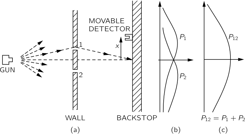
Fig. 37–1 Interference experiment with bullets.
To try to understand the quantum behavior of electrons, we shall compare and contrast their behavior, in a particular experimental setup, with the more familiar behavior of particles like bullets, and with the behavior of waves like water waves.
We consider first the behavior of bullets in the experimental setup shown diagrammatically in Fig. 37–1. We have a machine gun that shoots a stream of bullets. It is not a very good gun, in that it sprays the bullets (randomly) over a fairly large angular spread, as indicated in the figure. In front of the gun we have a wall (made of armor plate) that has in it two holes. Beyond the wall is a backstop (say a thick wall of wood) which will “absorb” the bullets when they hit it. In front of the wall we have an object which we shall call a “detector” of bullets. It might be a box containing sand. The detector can be moved back and forth (in what we will call the x-direction). With this apparatus, we can find out experimentally the answer to the question: “What is the probability that a bullet which passes through the holes in the wall will arrive at the backstop at the distance x from the center?” By “probability” we mean the chance that the bullet will arrive at the detector, which we can measure by counting the number which arrive at the detector in a certain time and then taking the ratio of this number to the total number that hit the backstop during that time. Bullets arrive in lumps, when we find something in the detector, it is always one whole bullet. We shall say: “Bullets always arrive in identical lumps.”
The result of such measurements with this apparatus (we have not yet done the experiment, so we are really imagining the result) are plotted in the graph drawn in part (c) of Fig. 37–1. In the graph we plot the probability to the right and x vertically, so that the x-scale fits the diagram of the apparatus. We call the probability  because the bullets may have come either through hole 1 or through hole 2. You will not be surprised that is large near the middle of the graph but gets small if x is very large. You may wonder, however, why has its maximum value at x=0. We can understand this fact if we do our experiment again after covering up hole 2, and once more while covering up hole 1. When hole 2 is covered, bullets can pass only through hole 1, and we get the curve marked
  in part (b) of the figure. As you would expect, the maximum of occurs at the value of x which is on a straight line with the gun and hole 1. When hole 1 is closed, we get the symmetric curve
  drawn in the figure. Comparing parts (b) and (c) of Fig. 37–1, we find the important result that
![[ P_{12}=P_1+P_2 ]](http://tlonworld.com/wp-content/ql-cache/quicklatex.com-beea263141f769bbf581df66c1213b9a_l3.svg "Rendered by QuickLaTeX.com")
The probabilities just add together. The effect with both holes open is the sum of the effects with each hole open alone. We shall call this result an observation of “no interference,” for a reason that you will see later. So much for bullets. They come in lumps, and their probability of arrival shows no interference.
An experiemnt with waves
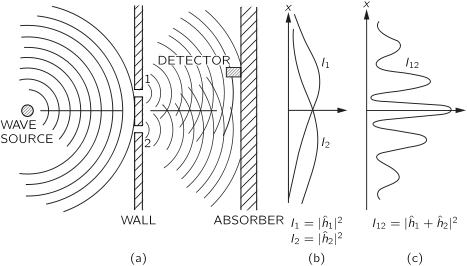
Fig. 37–2.Interference experiment with water waves.
Now we wish to consider an experiment with water waves. The apparatus is shown diagrammatically in Fig. 37–2. We have a shallow trough of water. A small object labeled the “wave source” is jiggled up and down by a motor and makes circular waves. To the right of the source we have again a wall with two holes, and beyond that is a second wall, which, to keep things simple, is an “absorber,” so that there is no reflection of the waves that arrive there. This can be done by building a gradual sand “beach.” In front of the beach we place a detector which can be moved back and forth in the xx-direction, as before. The detector is now a device which measures the “intensity” of the wave motion.
Now let us measure the wave intensity for various values of x (keeping the wave source operating always in the same way). We get the interesting-looking curve marked  in part (c) of the figure.
We have already worked out how such patterns can come about when we studied the interference of electric waves. In this case we would observe that the original wave is diffracted at the holes, and new circular waves spread out from each hole. If we cover one hole at a time and measure the intensity distribution at the absorber we find the rather simple intensity curves shown in part (b) of the figure.  is the intensity of the wave from hole 1 (which we find by measuring when hole 2 is blocked off) and
  is the intensity of the wave from hole 2 (seen when hole 1 is blocked).
The intensity observed when both holes are open is certainly not the sum of and . We say that there is “interference” of the two waves. At some places (where the curve has its maxima) the waves are “in phase” and the wave peaks add together to give a large amplitude and, therefore, a large intensity. We say that the two waves are “interfering constructively” at such places. There will be such constructive interference wherever the distance from the detector to one hole is a whole number of wavelengths larger (or shorter) than the distance from the detector to the other hole.
At those places where the two waves arrive at the detector with a phase difference of ππ(where they are “out of phase”) the resulting wave motion at the detector will be the difference of the two amplitudes. The waves “interfere destructively,” and we get a low value for the wave intensity. We expect such low values wherever the distance between hole 1 and the detector is different from the distance between hole 2 and the detector by an odd number of half-wavelengths.
The quantitative relationship between , and is the following. with  complex numbers.
![[ I_{12}=|h_1+h_2|^2=I_1+I_2+2 ,I_1, I_2, cosvarphi ]](http://tlonworld.com/wp-content/ql-cache/quicklatex.com-32cd261b08cad0d4e77f55368a511544_l3.svg "Rendered by QuickLaTeX.com")
with  the modulus square of the complex numbers and
  the relative phase between the two waves. You will notice that the result is quite different from that obtained with bullets (Eq. 37.1). The last term in (37.4) is the “interference term.” The intensity can have any value, and it shows interference.
An experiment with electrons
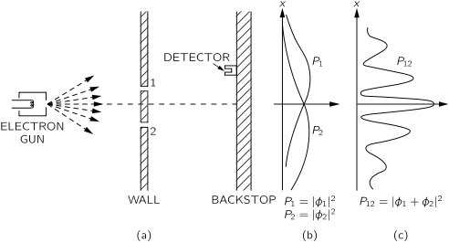
Fig. 37–3.Interference experiment with electrons.
Now we imagine a similar experiment with electrons. It is shown diagrammatically in Fig. 37–3. We make an electron gun which consists of a tungsten wire heated by an electric current and surrounded by a metal box with a hole in it. If the wire is at a negative voltage with respect to the box, electrons emitted by the wire will be accelerated toward the walls and some will pass through the hole. All the electrons which come out of the gun will have (nearly) the same energy. In front of the gun is again a wall (just a thin metal plate) with two holes in it. Beyond the wall is another plate which will serve as a “backstop.” In front of the backstop we place a movable detector. The detector might be a geiger counter or, perhaps better, an electron multiplier, which is connected to a loudspeaker. The first thing we notice with our electron experiment is that we hear sharp “clicks” from the detector (that is, from the loudspeaker). And all “clicks” are the same. There are no “half-clicks.”
As we move the detector around, the rate at which the clicks appear is faster or slower, but the size (loudness) of each click is always the same. If we lower the temperature of the wire in the gun the rate of clicking slows down, but still each click sounds the same. We would notice also that if we put two separate detectors at the backstop, one or the other would click, but never both at once. We conclude, therefore, that whatever arrives at the backstop arrives in “lumps.” All the “lumps” are the same size: only whole “lumps” arrive, and they arrive one at a time at the backstop. We shall say: “Electrons always arrive in identical lumps.”
Just as for our experiment with bullets, we can now proceed to find experimentally the answer to the question: “What is the relative probability that an electron ‘lump’ will arrive at the backstop at various distances x from the center?” As before, we obtain the relative probability by observing the rate of clicks, holding the operation of the gun constant. The result of our experiment is the interesting curve marked in part (c) of Fig. 37–3. The mathematics is the same as that we had for the water waves!
We conclude the following: The electrons arrive in lumps, like particles, and the probability of arrival of these lumps is distributed like the distribution of intensity of a wave. It is in this sense that an electron behaves “sometimes like a particle and sometimes like a wave.”
Watching the electrons
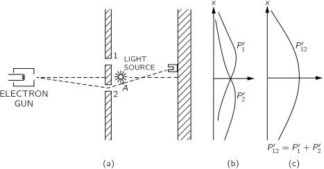
Fig. 37–4.A different electron experiment.
We shall now try the following experiment. To our electron apparatus we add a very strong light source, placed behind the wall and between the two holes, as shown in Fig. 37–4. We know that electric charges scatter light. So when an electron passes, however it does pass, on its way to the detector, it will scatter some light to our eye, and we can see where the electron goes.
Here is what we see: every time that we hear a “click” from our electron detector (at the backstop), we also see a flash of light either near hole 1 or near hole 2, but never both at once! And we observe the same result no matter where we put the detector. From this observation we conclude that when we look at the electrons we find that the electrons go either through one hole or the other. Still, when we succeeded in watching which hole our electrons come through, we no longer get the old interference curve but a new one showing no interference! If we turn out the light is restored.
We must conclude that when we look at the electrons the distribution of them on the screen is different than when we do not look. By trying to “watch” the electrons we have changed their motions.
You may be thinking: “Don’t use such a bright source! The light waves will then be weaker and will not disturb the electrons so much. As we turn down the intensity of the light source we change the rate at which they are emitted, so some electrons get by without being seen.
We learned in an earlier chapter that the momentum carried by a “photon” is inversely proportional to its wavelength. If we want to disturb the electrons only slightly we should lower its frequency (the same as increasing its wavelength). Let us use light of a redder color. Let us try the experiment with longer waves. At first, nothing seems to change. The results are the same. Then a terrible thing happens. You remember that when we discussed the microscope we pointed out that, due to the wave nature of the light, there is a limitation on how close two spots can be and still be seen as two separate spots. This distance is of the order of the wavelength of light. So now, when we make the wavelength longer than the distance between our holes, we see a big fuzzy flash when the light is scattered by the electrons. We can no longer tell which hole the electron went through! We just know it went somewhere! And it is just with light of this color that we find that the jolts given to the electron are small enough so that we begin to get some interference effect.
It was suggested by Heisenberg that the then new laws of nature could only be consistent if there were some basic limitation on our experimental capabilities not previously recognized. He proposed, as a general principle, his uncertainty principle, which we can state in terms of our experiment as follows: “It is impossible to design an apparatus to determine which hole the electron passes through, that will not at the same time disturb the electrons enough to destroy the interference pattern.”
First principles of Quantum mechanics
The probability of an event in an ideal experiment is given by the square of the absolute value of a complex number ? which is called the probability amplitude 
When an event can occur in several alternative ways, the probability amplitude for the event is the sum of the probability amplitudes for each way considered separately. There is interference: 
If an experiment is performed which is capable of determining whether one or another alternative is actually taken, the probability of the event is the sum of the probabilities for each alternative. The interference is lost:  .
.
The uncertainty principle
This is the way Heisenberg stated the uncertainty principle originally: If you make the measurement on any object, and you can determine the x-component of its momentum with an uncertainty ?p, you cannot, at the same time, know its x-position more accurately than
![[ Delta xgeq {hbarover 2 Delta p} ]](http://tlonworld.com/wp-content/ql-cache/quicklatex.com-0cd9fd93b08cba911bbd351ca91f5629_l3.svg "Rendered by QuickLaTeX.com")
The Kinetic Theory of gases
The pressure of a gas
We imagine that we have a volume of gas in a box, at one end of which is a piston which can be moved (Fig. 39–1). We would like to find out what force on the piston results from the fact that there are atoms in this box. One way of expressing the force is to talk about the force per unit area: if A is the area of the piston, then the force on the piston will be written as a number times the area. We define the pressure as the force per unit area
![[ P={Fover A} ]](http://tlonworld.com/wp-content/ql-cache/quicklatex.com-171bed9e0c4545d73d174110b8f2a678_l3.svg "Rendered by QuickLaTeX.com")
The differential work dW done on the gas in compressing it by moving the piston is then
![[ dW=F , (-dx)=-P, dV ]](http://tlonworld.com/wp-content/ql-cache/quicklatex.com-45042ed2ec843f06beb98721ac510125_l3.svg "Rendered by QuickLaTeX.com")
If  is the velocity of an atom in the direction of the piston, the total momentum delivered to the piston by a particle collision is
  , because it is “reflected.” The number of collisions in a time dt is equal to half the number of atoms which are in the region within a distance
  (the other half go in the opposite direction). Let N the total number of atoms in a volume
  , then the number of collisions against the piston is
  and the pressure
![[ P, V= N, m , langle v^2_x rangle =frac{2}{3} , U ]](http://tlonworld.com/wp-content/ql-cache/quicklatex.com-615a7cb398fdf6b17803cdbcf5a5b557_l3.svg "Rendered by QuickLaTeX.com")
with  is the total kinetic energy and
  the average square velocity. For somewhat wider generality, we shall write
![[ P, V=(1-gamma) U ]](http://tlonworld.com/wp-content/ql-cache/quicklatex.com-690b27787688284e14b00168e20e8a3b_l3.svg "Rendered by QuickLaTeX.com")
with  for a monoatomic gas. A compression in which there is no heat energy added or removed is called an adiabatic compression. For an adiabatic compression all the work done goes into changing the internal energy and therefore
  leading to
![[ P, V^gamma ={rm const} ]](http://tlonworld.com/wp-content/ql-cache/quicklatex.com-79b7813e431d4c5d137c37b0f3357030_l3.svg "Rendered by QuickLaTeX.com")
For a photon  and the atom kinetic energy
  is replaced by
  , so one finds
![[ P, V = {Uover 3} quad quad {rm photon~gas} ]](http://tlonworld.com/wp-content/ql-cache/quicklatex.com-859ddd3f5cfd1f3a7ef0b3a63b047a6e_l3.svg "Rendered by QuickLaTeX.com")
or equivalently  .
.
Temperature
The mean molecular kinetic energy is a property only of the “temperature.” Being a property of the “temperature,” and not of the gas, we can use it as a definition of the temperature. We say that the mean molecular kinetic energy is  with T the absolute temperature and
  Joule per degree Kelvin.
The ideal gas law
Now, of course, we can use our definition of temperature to find the law for the pressure of gases as a function of the temperature:
![[ P, V=N, k, T ]](http://tlonworld.com/wp-content/ql-cache/quicklatex.com-a877106f3f076b59a799b37a464550d2_l3.svg "Rendered by QuickLaTeX.com")
Furthermore, at the same temperature and pressure and volume, the number of atoms is determined.
The principles of statitical mechanics
The Boltzmann law
Here we study how are the molecules distributed in space when there are forces acting on them, and how are they distributed in velocity. Let us P be the pressure at height h. The vertical force per unit area pushing down at a height h+dh would be the same, in the absence of gravity, but in presence of gravity must exceed the force from above by the weight of gas in the section between h and h+dh. Now mg is the force of gravity on each molecule, where g is the acceleration due to gravity, and n=N/V the number of molecules per unit volume. If the temperature is constant one finds
![[ dP=dn , k , T=-m ,g ,n ,dh ]](http://tlonworld.com/wp-content/ql-cache/quicklatex.com-33ca028f56f28a9ade31844a0128f56b_l3.svg "Rendered by QuickLaTeX.com")
solving for the density n one finds
![[n=n_0 , e^{-{Eover kT}} ]](http://tlonworld.com/wp-content/ql-cache/quicklatex.com-d567a27f46b931445bba8db7a9d03047_l3.svg "Rendered by QuickLaTeX.com")
with  the potential energy of an atom. One can show that this proposition is true for any conservative law. For example, the molecules may be charged electrically, and may be acted on by an electric field or another charge that attracts them. The equation above, known as Boltzmann’s law, states that the probability of finding molecules in a given spatial arrangement varies exponentially with the negative of the potential energy of that arrangement, divided by kT.
Similarly, the density  of molecules with a given kinetic energy
  is
is
![[n_{v}=n_0 , e^{-{E_vover kT}} ]](http://tlonworld.com/wp-content/ql-cache/quicklatex.com-1bc95be3ab1a95dbec2c3477f876377c_l3.svg "Rendered by QuickLaTeX.com")
The specific heats of gases
We have seen that a monatomic gas like Helium has . But suppose it is, say, a more complicated molecule. What about a gas made of diatomic molecules. We know that for each of the two atoms, each of the kinetic energies should be 3kT/2. In addition we have the vibration energy due to the fact that the two atoms are bounded by an attractive force. To an excellent approximation, the molecule can be represented as two atoms connected by a spring.. The potential energy of a harmonic oscillator equals the average kinetic energy and therefore the potential energy of vibration is kT/2. The grand total of energy is therefore U=7kT/2 leading to  .
.
The failure of classical physics
We might try some force law other than a spring, but it turns out that anything else will only make higher. If we include more forms of energy, approaches unity more closely, contradicting the facts. The fact is that there are electrons in each atom, and we know from their spectra that there are internal motions; each of the electrons should have at least kT/2 of kinetic energy, and something for the potential energy, so when these are added in, γ gets still smaller. It is wrong.
The first great paper on the dynamical theory of gases was by Maxwell in 1859. On the basis of ideas we have been discussing, he was able accurately to explain a great many known relations, such as Boyle’s law, the diffusion theory, the viscosity of gases, and things we shall talk about later. He listed all these great successes in a final summary, and at the end he said, “Finally, by establishing a necessary relation between the motions of translation and rotation (he is talking about the kT/2 theorem) of all particles not spherical, we proved that a system of such particles could not possibly satisfy the known relation between the two specific heats.”
Ten years later, in a lecture, he said, “I have now put before you what I consider to be the greatest difficulty yet encountered by the molecular theory.” These words represent the first discovery that the laws of classical physics were wrong.
Without proof, we may state the results for statistical mechanics of the quantum-mechanical theory. The simple result we have in classical mechanics, that  becomes the following very important theorem: If the energies of the set of molecular states are called, say,
  , then in thermal equilibrium the probability of finding a molecule in the particular state of having energy
  is
is  . So it is less likely to be in a higher energy state than in a lower one.
Now it turns out that for a harmonic oscillator the energy levels are evenly spaced  . Now suppose that kT is much less than ℏω. Then the probability of its being in state different from the ground state is extremely small. Practically all the atoms are in the ground state. All oscillators are in the bottom state, and their motion is effectively “frozen”; there is no contribution of it to the specific heat.
We have been discussing the properties of matter from the atomic point of view, trying to understand roughly what will happen if we suppose that things are made of atoms obeying certain laws. However, there are a number of relationships among the properties of substances which can be worked out without consideration of the detailed structure of the materials. The determination of the relationships among the various properties of materials, without knowing their internal structure, is the subject of thermodynamics.
We know from the kinetic theory that the pressure of a gas is caused by molecular bombardment, and we know that if we heat a gas, so that the bombardment increases, the pressure must increase. If we increase the temperature at a given volume, we increase the pressure and if we compress the gas, we will find that the temperature will rise. From the kinetic theory, one can derive a quantitative relationship between these two effects, but instinctively one might guess that they are related in some necessary fashion which is independent of the details of the collisions.
The science of thermodynamics began with an analysis, by the great engineer Sadi Carnot, of the problem of how to build the best and most efficient engine.
Now the way a steam engine ordinarily operates is that heat from a fire boils some water, and the steam so formed expands and pushes on a piston which makes a wheel go around, then the steam go into another box, where it is condensed by cool water, and then pump the water back into the boiler, so that it circulates continuously. Heat is thus supplied to the engine and converted into work. Now would it be better to use alcohol? What property should a substance have so that it makes the best possible engine? That was the question to which Carnot addressed himself.
The results of thermodynamics are all contained implicitly in certain apparently simple statements called the laws of thermodynamics. The first law states the conservation of energy: The heat Q put into the system, plus the work W done on the system, is the increase in the energy U of the system; the latter energy is sometimes called the internal energy:
![[ Delta U=Delta Q+Delta W ]](http://tlonworld.com/wp-content/ql-cache/quicklatex.com-60d6590d61f4e49d83fc90e65f2bd8a6_l3.svg "Rendered by QuickLaTeX.com")
We know that if we do work against friction, say, the work lost to us is equal to the heat produced. If we do work in a room at temperature T, and we do the work slowly enough, the room temperature does not change much, and we have converted work into heat at a given temperature. What about the reverse possibility? Is it possible to convert the heat back into work at a given temperature? The second law of thermodynamics asserts that it is not. The heat cannot be taken in at a certain temperature and converted into work with no other change in the system or the surroundings. Heat cannot, of itself, flow from a cold to a hot object.
Reversible engines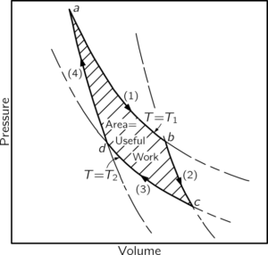
Suppose that we have a gas in a cylinder equipped with a frictionless piston. Also, suppose that we have two heat pads, that have definite temperatures  and
and  . We will suppose in this case that
  . Let us first heat the gas and at the same time expand it pulling the piston out very slowly. We then push the piston back slowly keeping fix the temperature so the heat would pour back. We see that such an isothermal (constant-temperature) expansion, done slowly and gently enough, is a reversible process.
For an ideal gas  . During an isothermal expansion the pressure falls as the volume increases until we stop at the point b. At the same time, a certain heat
  must flow into the gas from the reservoir. Having completed the isothermal expansion, stopping at the point b, let us take the cylinder away from the reservoir and continue the expansion. This time we permit no heat to enter the cylinder. Again we perform the expansion slowly, so there is no reason why we cannot reverse it, and we again assume there is no friction. The gas continues to expand and the temperature falls, since there is no longer any heat entering the cylinder. We let the gas expand, following the curve marked (2), until the temperature falls to . This kind of expansion, made without adding heat, is called an adiabatic expansion.
For an ideal gas, we already know that curve (2) has the form PVγ=constant, where γ is a constant greater than 1, so that the adiabatic curve has a more negative slope than the isothermal curve. The gas cylinder has now reached the temperature T2, so that if we put it on the heat pad at temperature T2 there will be no irreversible changes. Now we slowly compress the gas while it is in contact with the reservoir at T2, following the curve marked (3). Because the cylinder is in contact with the reservoir, the temperature does not rise, but heat Q2 flows from the cylinder into the reservoir at the temperature T2. Having compressed the gas isothermally along curve (3) to the point d, we remove the cylinder from the heat pad at temperature T2 and compress it still further, without letting any heat flow out. The temperature will rise, and the pressure will follow the curve marked (4). If we carry out each step properly, we can return to the point a at temperature T1
For an ideal gas, we already know that curve (2) has the form  where γ is a constant greater than 1, so that the adiabatic curve has a more negative slope than the isothermal curve. The gas cylinder has now reached the temperature , so that if we put it on the heat pad at temperature there will be no irreversible changes. Now we slowly compress the gas while it is in contact with the reservoir at , following the curve marked (3). Because the cylinder is in contact with the reservoir, the temperature does not rise, but heat
  flows from the cylinder into the reservoir at the temperature . Having compressed the gas isothermally along curve (3) to the point d, we remove the cylinder from the heat pad at temperature and compress it still further, without letting any heat flow out. The temperature will rise, and the pressure will follow the curve marked (4). If we carry out each step properly, we can return to the point a at temperature where we started, and repeat the cycle.
Now the point is that this cycle is reversible, so that we could represent all the steps the other way around. We could have gone backwards instead of forwards.
If we go around the cycle in one direction, we must do work on the gas; if we go in the other direction, the gas does work on us.
Incidentally, it is easy to find out what the total amount of work is, because the work during any expansion is the pressure times the change in volume,
 , in other words, the area under the curve. So the area under each of the numbered curves is a measure of the work done by or on the gas in the corresponding step. It is easy to see that the network done is the shaded area of the picture.
If an engine is reversible, the amount of work one will obtain if the engine absorbs a given amount of heat at temperature and delivers heat at some other temperature does not depend on the design of the engine. It is a property of the world, not a property of a particular engine.
The efficiency of ideal gas engines
Let us compute now the heats and exchanges along a Carnot cycle. We have
![[ Q_1=int_a^b p, dV=N, k, T_1 int_a^b {dVover V} =N, k, T_1 , ln{V_bover V_a} ]](http://tlonworld.com/wp-content/ql-cache/quicklatex.com-1290a9a8f54aca274f46fe8f2b95cbe6_l3.svg "Rendered by QuickLaTeX.com")
Similarly  . On the other hand along the adiabatic expansion curve
![[ T_1, V_b^{gamma-1}=T_2, V_c^{gamma-1} quadquad T_1, V_a^{gamma-1}=T_2, V_d^{gamma-1} ]](http://tlonworld.com/wp-content/ql-cache/quicklatex.com-049eccbcb6153ab59056efe806ffc1d8_l3.svg "Rendered by QuickLaTeX.com")
Altogether one finds
![[ {Q_1over T_1}={Q_2over T_2} ]](http://tlonworld.com/wp-content/ql-cache/quicklatex.com-47211db3c2d95114a880d1b7c0eefe44_l3.svg "Rendered by QuickLaTeX.com")
This is the relation we were seeking. Although proved for a perfect gas engine, we know it must be true for any reversible engine at all.
The efficiency of an engine is defined as
![[ {rm Efficiency}={Q_1-Q_2over Q_1}=1-{T_2over T_1} <1 ]](http://tlonworld.com/wp-content/ql-cache/quicklatex.com-a4f448b6568cb5aa88d121a6fa785b56_l3.svg "Rendered by QuickLaTeX.com")
The entropy of a system  (or its increase) is defined as the amount of heat reversibly added to a system at a constant temperature , i.e.
Summary of Thermodynamics laws
The three theremodynamics was can then be states as of
First law: The energy of the universe is always constant.
Second law: The entropy of the universe is always increasing. A process whose only net result is to take heat from a reservoir and convert it to work is impossible. No heat engine taking heat from and delivering heat at can do more work than a reversible engine, for which
![[ W=Q_1-Q_2= Q_1, left({T_1-T_2over T_1}right) ]](http://tlonworld.com/wp-content/ql-cache/quicklatex.com-3dabd00045d4741455ddae52ed9078d5_l3.svg "Rendered by QuickLaTeX.com")
Third law: At  ,
,  .
.
In a reversible change, the total entropy of all parts of the system (including reservoirs) does not change. In irreversible change, the total entropy of the system always increases.
 The Hit (Frears, 1984)
 Frankenstein (1931, dir. James Whale)
 Ashes and Diamonds (1958, Andrzej Wajda)
 The Tree of Wooden Clogs(1978, E.Olmi)
  8 1/2 (1963, dir. Federico Fellini)
 1. I Vitelloni (Fellini, 1953)
 The Good, the Bad and the Ugly (1966, dir. Sergio Leone)