Dogs , Cows and cabbages
The dead hand of plato
 Biology, according to Mayr, is plagued by its own version of essentialism. Biological essentialism treats tapirs and rabbits, pangolins and dromedaries, as though they were triangles, rhombuses, parabolas or dodecahedrons. The rabbits that we see are wan shadows of the perfect ‘idea’ of rabbit, the ideal, essential, Platonic rabbit, hanging somewhere out in conceptual space along with all the perfect forms of geometry. Flesh-and-blood rabbits may vary, but their variations are always to be seen as flawed deviations from the ideal essence of rabbit.
How desperately unevolutionary that picture is! The Platonist regards any change in rabbits as a messy departure from the essential rabbit, and there will always be resistance to change – as if all real rabbits were tethered by an invisible elastic cord to the Essential Rabbit in the Sky. The evolutionary view of life is radically opposite. Descendants can depart indefinitely from the ancestral form, and each departure becomes a potential ancestor to future variants. Indeed, Alfred Russel Wallace, independent codiscoverer with Darwin of evolution by natural selection, actually called his paper ‘On the tendency of varieties to depart indefinitely from the original type’.
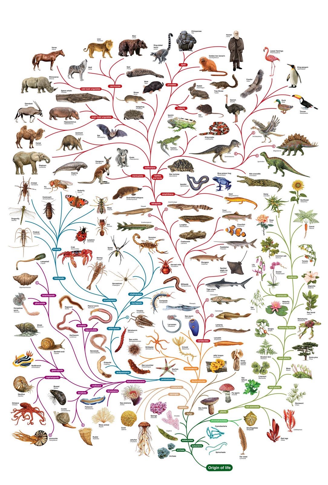
For any two animals there has to be a hairpin path linking them, for the simple reason that every species shares an ancestor with every other species: all we have to do is walk backwards from one species to the shared ancestor, then turn through a hairpin bend and walk forwards to the other species. We are talking only about locating a chain of animals that links a modern animal to another modern animal. We are most emphatically not evolving a rabbit into a leopard. Modern species don’t evolve into other modern species, they just share ancestors: they are cousins.
However radical and extensive the differences between the ends of the hairpin – rabbit and leopard, say – each step along the chain that links them is very, very small. Every individual along the chain is as similar to its neighbours in the chain as mothers and daughters are expected to be.
 Sculpting the gene pool
Cabbages are a vegetable affront to essentialism and the immutability of species. The wild cabbage, Brassica oleracea, is an undistinguished plant, vaguely like a weedy version of a domestic cabbage. In just a few centuries, wielding the fine and coarse chisels furnished by the toolbox of selective breeding techniques, horticulturalists have sculpted this rather nondescript plant into vegetables as strikingly different from each other and from the wild ancestor as broccoli, cauliflower, kohlrabi, kale, Brussels sprouts, spring greens, romanescu and, of course, the various kinds of vegetables that are still commonly called cabbage.
The relevance to natural evolution is that, although the selecting agent is man and not nature, the process is otherwise exactly the same. This is why Darwin gave so much prominence to domestication at the beginning of On the Origin of Species. Anybody can understand the principle of evolution by artificial selecti
on. Natural selection is the same, with one minor detail changed.
A Mendelian gene is an all-or-nothing entity. When you were conceived, what you received from your father was not a substance, to be mixed with what you received from your mother as if mixing blue paint and red paint to make purple. If this were really how heredity worked (as people vaguely thought in Darwin’s time) we’d all be a middling average, halfway between our two parents. In that case, all variation would rapidly disappear from the population (no matter how assiduously you mix purple paint with purple paint, you’ll never reconstitute the original red and blue). In fact, of course, any
body can plainly see that there is no such intrinsic tendency for variation to decrease in a population. Mendel showed that this is because when paternal genes and maternal genes are combined in a child (he didn’t use the word ‘gene’, which wasn’t coined until 1909), it is not like blending paints, it is more like shuffling and reshuffling cards in a pack. Nowadays, we know that genes are lengths of DNA code, not physically separate like cards, but the principle remains valid. Genes don’t blend; they shuffle.
Any one of your eggs (or sperms if you are male) contains either your father’s version of a particular gene or your mother’s version, not a blend of the two. And that particular gene came from one and only one of you
r four grandparents; and from one and only one of your eight great-grandparents.
A sexually reproducing population, such as, say, all the rats on Ascension Island, remotely isolated in the South Atlantic, is continually shuffling all the genes on the island. There is no intrinsic tendency for each generation to become less variable than the previous generation, no tendency towards ever more boringly grey, middling intermediates. The genes remain intact, shuffled about from individual body to individual body as the generations go by, but not blending with one another, never contaminatin
g each other.
There is no intrinsic tendency in gene pools for particular genes to increase or decrease in frequency. But when there is a systematic increase or decrease in the frequency with which we see a particular gene in a gene pool, that is precisely and exactly what is meant by evolution.
Mutations are the random changes in genes that constitute the raw material for evolution by non-random selection.
Without any understanding at all, just by choosing who mates with whom, you can breed for all kinds of desired characteristics. This is what dog breeders, and animal and plant breeders generally, achieved for centuries before anybody understood anything about genetics. And there’s a lesson in that about nat
ural selection, for nature, of course, has no understanding or awareness of anything at all.
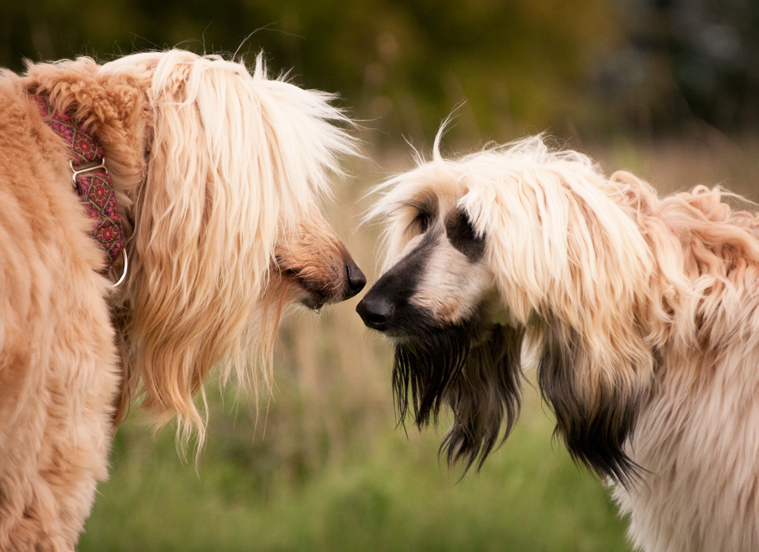
First, the great variety among breeds of dogs, from Great Danes to Yorkies, from Scotties to Airedales, from ridgebacks to dachshunds, from whippets to St Bernards, demonstrates how easy it is for the non-random selection of genes – the ‘carving and whittling’ of gene pools – to produce truly dramatic changes in anatomy and behaviour, and so fast.
 Insects were the first domesticators
‘Mammoth’ sunflowers, originally bred in Russia, are 12 to 17 feet high, the head diameter is close to one foot, which is more than ten times the size of a wild sunflower’s disc, and there is normally only one head per plant, instead of the many, much smaller, flowers of the wild plant. The Russians started breeding this American flower, by the way, for religious reasons. During Lent and Advent, the use of oil in cooking was banned by the Orthodox Church. Conveniently, and for a reason that I – untutored in the profundities of theology – shall not presume to fathom, sunflower seed oil was deemed to be exempt from this prohibition. This provided one of the economic pressures that drove the recent selective breeding of the sunflower. Long before the modern era, however, native Americans had been cultivating these nutritious and spectacular flowers for food, for dyes and for decoration, and they achieved results intermediate between the wild sunflower and the extravagant extremes of modern cultivars. But before that again, sunflowers, like all brightly coloured flowers, owed their very existence to selective breeding by insects.
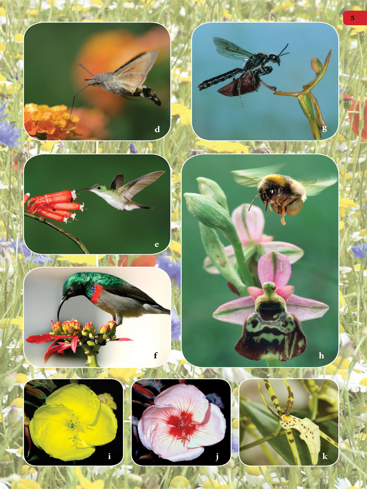
Generations of ancestral flowers were chosen by generations of ancestral insects or hummingbirds or other natural pollinators. It is a perfectly good example of selective breeding, with the minor difference that the breeders were insects and hummingbirds, not humans.
It is of the essence of sexual reproduction that you shouldn’t fertilize yourself. Pollen must somehow be transported from one plant to another. Hermaphroditic plants that have male and female parts within one flower often go to elaborate lengths to stop the male half from fertilizing the female half.
Pollen is a fine, light powder. If you release enough of it on a breezy day, one or two grains may have the luck to land on the right spot in a flower of the right species. But wind pollination is wasteful. The vast majority of pollen grains land somewhere other than where they should, and all that energy and costly matériel is wasted. There is a more directed way for pollen to be targeted. Nectar is sugary syrup, and it is manufactured by plants specifically and only for paying, and fuelling, bees, butterflies, hummingbirds, bats and other hired transport.
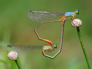
Both Darwin and his co-discoverer of natural selection, Wallace, called attention to an amazing orchid from Madagascar, Angraecum sesquipedale and both men made the same remarkable prediction, which was later triumphantly vindicated. This orchid has tubular nectaries that reach down more than 11 inches by Darwin’s own ruler. That’s nearly 30 centimetres. A related species, Angraecum longicalcar, has nectar-bearing spurs that are even longer, up to 40 centimetres (more than 15 inches). Darwin, purely on the strength of A. sesquipedale’s existence in Madagascar, predicted in his orchid book of 1862 that there must be ‘moths capable of extension to a length of between ten and eleven inches’. Wallace, five years later (it isn’t clear whether he had read Darwin’s book) mentioned several moths whose probosces were nearly long enough to meet the case.
Insects have good colour vision, but their whole spectrum is shifted towards the ultraviolet and away from the red. Like us, they see yellow, green, blue and violet. Unlike us, however, they also see well into the ultraviolet range; and they don’t see red, at ‘our’ end of the spectrum. If you have a red tubular flower in your garden it is a good bet, though not a certain prediction, that in the wild it is pollinated not by insects but by birds, who see well at the red end of the spectrum – perhaps hummingbirds if it is a New World plant, or sunbirds if an Old World plant. Flowers that look plain to us may actually be lavishly decorated with spots or stripes for the benefit of insects, ornamentation that we can’t see because we are blind to ultraviolet.
This floral extravaganza, splashed across the green canvas of a meadow, has been shaped and coloured, magnified and titivated by the past choices made by animal eyes: bee eyes, butterfly eyes, hoverfly eyes. In New World forests we’d have to add hummingbird or in African forests sunbird eyes to the list. Hummingbird eyes, hawk-moth eyes, butterfly eyes, hoverfly eyes, bee eyes are critically cast over wild flowers, generation after generation, shaping them, colouring them, swelling them, patterning and stippling them, in almost exactly the same way as human eyes later did with our garden varieties; and with dogs, cows, cabbages and corn.
For the flower, insect pollination represents a huge advance in economy over the wasteful scattergun of wind pollination. Even if a bee visits flowers indiscriminately, lurching promiscuously from buttercup to cornflower, from poppy to celandine, a pollen grain clinging to its hairy abdomen has a much greater chance of hitting the right target – a second flower of the same species – than it would have if scattered on the wind. Slightly better would be a bee with a preference for a particular colour, say blue. Or a bee that, while not having any long-term colour preference, tends to form colour habits, so that it chooses colours in runs. Better still would be an insect that visits flowers of only one species. And there are flowers, like the Madagascar orchid that inspired the Darwin/Wallace prediction, whose nectar is available only to certain insects that specialize in that kind of flower and benefit from their monopoly over it. Those Madagascar moths are the ultimate magic bullets.
From a moth’s point of view, flowers that reliably provide nectar are like docile, productive milch cows. From the flowers’ point of view, moths that reliably transport their pollen to other flowers of the same species are like a well-paid Federal Express service, or like well-trained homing pigeons. Each side could be said to have domesticated the other, selectively breeding them to do a better job than they previously did. Human breeders of prize roses have had almost exactly the same kinds of effects on flowers as insects have – just exaggerated them a bit. Insects bred flowers to be bright and showy. Gardeners made them brighter and showier still. Insects made roses pleasantly fragrant. We came along and made them even more so. Incidentally, it is a fortunate coincidence that the fragrances that bees and butterflies prefer happen to appeal to us too.
The insects, by choosing the most attractive flowers to visit, inadvertently ‘breed for’ floral beauty. At the same time, the flowers are breeding the insects for pollination ability. Then again, I have implied that insects breed flowers for high nectar yield, like dairymen breeding massively uddered Friesians. But it is in the flowers’ interests to ration their nectar. Satiate an insect and it has no incentive to go on and look for a second flower – bad news for the first flower, for which the second visit, the pollinating visit, is the whole point of the exercise. From the flowers’ point of view, a delicate balance must be struck between providing too much nectar (no visit to a second flower) and too little (no incentive to visit the first flower).
 You are my natural selection
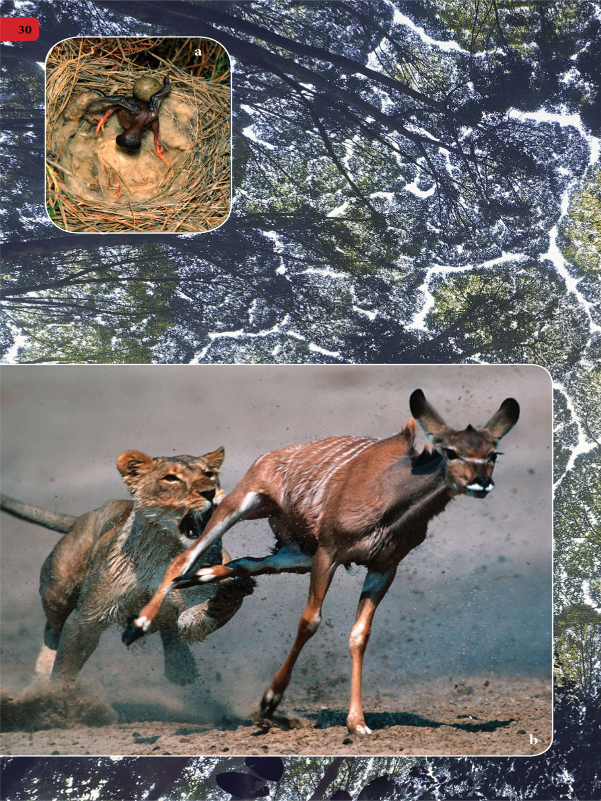
Bright colours may indeed attract predators, but they attract female pheasants too. Generations of hens chose to mate with bright, glowing males, rather than the dull brown creatures that the males would surely have remained but for selective breeding by females. The same thing happened with peahens selectively breeding peacocks, female birds of paradise breeding males, and numerous other examples of birds, mammals, fish, amphibians, reptiles and insects where females (it’s usually females rather than males) choose from among competing males.
Deep-sea angler fish sit on the bottom of the sea, waiting patiently for prey. Like many deep-sea fish, anglers are spectacularly ugly by our standards. May be by fish standards too, although it probably doesn’t matter because, down where they live, it is too dark to see much anyway. Like other denizens of the deep sea, female angler fish often make their own light – or rather, they have special receptacles in which they house bacteria which make light for them. Such ‘bioluminescence’ isn’t bright enough to reflect any detail, but it is bright enough to attract other fish. A spine becomes elongated and stiffened to make a fishing rod. On the end of the fishing rod is a bait, or lure. The baits vary from species to species, but they always resemble small food items: perhaps a worm, or a small fish, or just a nondescript but temptingly jiggling morsel. Often the bait is actually luminous: another natural neon sign, and in this case the message being flashed is ‘come and eat me’. Small fish are indeed tempted. They approach close to the bait. And it is the last thing they do for, at that moment, the angler opens her huge maw and the prey is engulfed with the inrush of water. The prey fish are indeed choosing the most ‘attractive’ angler fish for breeding, via the indirect route of choosing them for survival by feeding them! Anglers with unattractive lures are more likely to starve to death and therefore less likely to breed. And the small prey fish are indeed doing the ‘choosing’. But they are choosing with their lives!
It was Darwin who first spotted that you don’t have to have a choosing agent. The choice can be made automatically by survival – or failure to survive. Those individuals that are ‘chosen’ by the fact that they happen to possess superior equipment to survive are the most likely to reproduce, and therefore to pass on the genes for possessing superior equipment. Therefore every gene pool, in every species, tends to become filled with genes for making superior equipment for survival and reproduction. The general case is the non-random survival of randomly varying hereditary equipment.
It may be said that natural selection is daily and hourly scrutinising, throughout the world, every variation, even the slightest; rejecting that which is bad, preserving and adding up all that is good; silently and insensibly working, whenever and wherever opportunity offers, at the improvement of each organic being in relation to its organic and inorganic conditions of life. We see nothing of these slow changes in progress, until the hand of time has marked the long lapse of ages, and then so imperfect is our view into long past geological ages, that we see only that the forms of life are now different from what they formerly were.
Wallace went on to quote a French author called Janet, who was evidently, unlike Wallace and Darwin, a deeply muddled individual:
I see that he considers your weak point to be that you do not see that ‘thought and direction are essential to the action of Natural Selection.’ The same objection has been made a score of times by your chief opponents, and I have heard it as often stated myself in conversation. Now, I think this arises almost entirely from your choice of the term Natural Selection, and so constantly comparing it in its effects to man’s selection, and also to your so frequently personifying nature as ‘selecting’, as ‘preferring’ . . . etc., etc. To the few this is as clear as daylight, and beautifully suggestive, but to many it is evidently a stumbling-block. I wish, therefore, to suggest to you the possibility of entirely avoiding this source of misconception in your great work, and also in future editions of the ‘Origin,’ and I think it may be done without difficulty and very effectually by adopting Spencer’s term . . . ‘Survival of the Fittest.’ This term is the plain expression of the fact; ‘Natural Selection’ is a metaphorical expression of it . . .
Experimental interference is of enormous importance, because without it you can never be sure that a correlation you observe has any causal significance. This can be illustrated by the so-called ‘church clocks fallacy’. The clocks in the towers of two neighbouring churches chime the hours, but St A’s a little before St B’s. A Martian visitor, noting this, might infer that St A’s chime caused St B’s to chime. It is only experimental manipulation that can determine whether an observed correlation truly indicates causation.
Artificial selection is not just an analogy for natural selection. Artificial selection constitutes a true experimental – as opposed to observational – test of the hypothesis that selection causes evolutionary change.
Rat's teeths
We can expect bodies to be well equipped to survive, but this does not mean they should be perfect with respect to any one dimension. It might seem obvious that tooth decay is to be avoided at all costs, and I do not doubt that dental caries significantly shortens life in rats. But let’s think for a moment about what must happen in order to increase an animal’s resistance to tooth decay. Let us suppose it is achieved by a thickening of the wall of the tooth, and this requires extra calcium. It is not impossible to find extra calcium, but it has to come from somewhere, and it is not free. Calcium (or whatever the limiting resource might be) is not floating around in the air. It has to come into the body via food. And it is potentially useful for other things apart from teeth. The body has something we could call a calcium economy. Calcium is needed in bone, and it is needed in milk. An individual rat with extra strong teeth might well tend to live longer than a rat with rotten teeth, all other things being equal. But all other things are not equal, because the calcium needed to strengthen the teeth had to come from somewhere, say, bones. A rival individual whose genes did not predispose it to take calcium away from bones might consequently survive longer, because of its superior bones and in spite of its bad teeth. Or the rival individual might be better qualified to rear children because she makes more calcium-rich milk. As economists are fond of quoting from Robert Heinlein, there’s no such thing as a free lunch. My rat example is hypothetical, but it is safe to say that, for economic reasons, there must be such a thing as a rat whose teeth are too perfect. Perfection in one department must be bought, in the form of a sacrifice in another department.
An antelope might run faster, and be more likely to escape a leopard, if its legs were a little longer. But a rival antelope with longer legs, although it might be better equipped to outsprint a predator, has to pay for its long legs in some other department of the body’s economy. The materials needed to make the extra bone and muscle in the longer legs have to be taken from somewhere else, so the longer-legged individual is more likely to die for reasons other than predation. Or it may even be more likely to die from predation because its longer legs, although they can run faster when intact, are more likely to break, in which case it can’t run at all. A body is a patchwork of compromises.
What happens under domestication is that animals are artificially shielded from many of the risks that shorten the lives of wild animals. A pedigree dairy cow may yield prodigious quantities of milk, but its pendulously cumbersome udder would seriously impede it in any attempt to outrun a lion. Thoroughbred horses are superb runners and jumpers, but their legs are vulnerable to injury during races, especially over jumps, which suggests that artificial selection has pushed them into a zone that natural selection would not have tolerated.
 Dogs again
If you see an animal feeding, you can measure its flight distance by seeing how close it will let you approach before fleeing. For any given species in any given situation, there will be an optimal flight distance, somewhere between too risky or foolhardy at the short end, and too flighty or risk-averse at the long end. We are puzzled when we see zebras or antelopes calmly grazing in full view of lions, keeping no more than a wary eye on them. They had to balance the risk of being eaten against the risk of not eating.
Much of the initial domestication of the dog was self- domestication, mediated by natural, not artificial, selection. We can imagine wild wolves scavenging on a rubbish tip on the edge of a village. Most of them, fearful of men throwing stones and spears, have a very long flight distance. They sprint for the safety of the forest as soon as a human appears in the distance. But a few individuals, by genetic chance, happen to have a slightly shorter flight distance than the average. Their readiness to take slight risks – they are brave, shall we say, but not foolhardy – gains them more food than their more risk-averse rivals. As the generations go by, natural selection favours a shorter and shorter flight distance, until just before it reaches the point where the wolves really are endangered by stone-throwing humans. The optimum flight distance has shifted because of the newly available food source.
The Russian geneticist Dimitri Belyaev was employed to run a fox fur farm in the 1950s. He was later sacked because his scientific genetics conflicted with the anti-scientific ideology of Lysenko, the charlatan biologist who managed to capture the ear of Stalin and so take over, and largely ruin, all of Soviet genetics and agriculture for some twenty years. Belyaev retained his love of foxes, and of true Lysenko-free genetics, and he was later able to resume his studies of both, as director of an Institute of Genetics in Siberia. Wild foxes are tricky to handle, and Belyaev set out deliberately to breed for tameness.
The cubs were classified into three classes. Class III cubs were those that fled from or bit the person. Class II cubs would allow themselves to be handled, but showed no positive responsiveness to the experimenters. Class I cubs, the tamest of all, positively approached the handlers, wagging their tails and whining. When the cubs grew up, the experimenters systematically bred only from this tamest class.
After a mere six generations of this selective breeding for tameness, the foxes had changed so much that the experimenters felt obliged to name a new category, the ‘domesticated elite’ class, which were ‘eager to establish human contact, whimpering to attract attention and sniffing and licking experimenters like dogs’. At the beginning of the experiment, none of the foxes were in the elite class. After ten generations of breeding for tameness, 18 per cent were ‘elite’; after twenty generations, 35 per cent; and after thirty to thirty-five generations, ‘domesticated elite’ individuals constituted between 70 and 80 per cent of the experimental population.
The tame foxes not only behaved like domestic dogs, they looked like them. They lost their foxy pelage and became piebald black and white, like Welsh collies. Their foxy prick ears were replaced by doggy floppy ears. Their tails turned up at the end like a dog’s, rather than down like a fox’s brush. The females came on heat every six months like a bitch, instead of every year like a vixen.
These dog-like features were side-effects. Belyaev and his team did not deliberately breed for them, only for tameness. This widespread phenomenon is called ‘pleiotropy’, whereby genes have more than one effect, seemingly unconnected.
 Flowers again
There are orchids that resemble female bees (or wasps or flies) well enough to fool males into attempting to copulate with them. The so-called spider orchid, Brassia, achieves pollination by a different kind of deception. The females of various species of solitary wasp (‘solitary’ because they don’t live socially in large nests like the familiar autumn pests, called yellow jackets by Americans) capture spiders, sting them to paralyse them, and lay their eggs on them as a living food supply for their larvae. Spider orchids resemble spiders sufficiently to fool female wasps into attempting to sting them. In the process they pick up pollinia – masses of pollen grains produced by the orchids. When they move on to try to sting another spider orchid, the pollinia are transferred. By the way, I can’t resist adding the exactly backwards case of the spider Epicadus heterogaster, which mimics an orchid. Insects come to the ‘flower’ in search of nectar, and are promptly eaten by it.
A male Euglossine bee is attracted to the orchids by the smell of the substances that he needs in order to manufacture his sexual perfumes. He alights on the rim of the bucket and starts to scrape the waxy perfume into the special scent pockets in his legs. But the rim of the bucket is slippery underfoot – and there’s a reason for this. The bee falls into the bucket, which is filled with liquid, in which he swims. He cannot climb up the slippery sides of the bucket. There is only one escape route, and this is a special bee- sized hole in the side of the bucket (not visible in the picture that appears on colour page 4). He is guided by ‘stepping stones’ to the hole and starts to crawl through it. It’s a tight fit, and it becomes even tighter as the ‘jaws’ (these you can see in the picture: they look like the chuck of a lathe or electric drill) contract and trap him. While he is held in their grip, they glue two pollinia to his back. The glue takes a while to set, after which the jaws again relax and release the bee, who flies off, complete with pollinia on his back. Still in search of the precious ingredients for his perfumery, the bee lands on another bucket orchid and the process repeats itself. This time, however, as the bee struggles through the hole in the bucket, the pollinia are scraped off, and they fertilize the stigma of this second orchid.
Silence and slow time
The measured age of our planet is about 4.6 billion years, or about 46 million centuries. The time that has elapsed since the common ancestor of all today’s mammals walked the Earth is about two million centuries.
To investigate evolution we don’t need just a clock that tells the present time, as a sundial does, or a watch. We need something more like a stopwatch that can be reset. Our evolutionary clock needs to be zeroed at some point, so that we can calculate the elapsed time since a starting point, to give us, for example, the absolute age of some object such as a rock. Radioactive clocks for dating igneous (volcanic) rocks are conveniently zeroed at the moment the rock is formed by the solidification of molten lava.
Fortunately, a variety of zero-able natural clocks is available. This variety is a good thing, because we can use some clocks to check the accuracy of other clocks. Even more fortunately, they sensitively cover an astonishingly wide range of timescales, and we need this too because evolutionary timescales span seven or eight orders of magnitude.
Radioactive decay clocks are available for short timescales as well, even down to fractions of a second; but for evolutionary purposes, clocks that can measure centuries or perhaps decades are about the fastest we need.
 Tree rings
A tree-ring clock can be used to date a piece of wood, say a beam in a Tudor house, with astonishing accuracy, literally to the nearest year. You can age a newly felled tree by counting rings in its trunk, assuming that the outermost ring represents the present. Rings represent differential growth in different seasons of the year – winter or summer, dry season or wet season.
But just counting rings doesn’t tell you in which century your house beam was alive, or your Viking longship’s mast. If you want to pin down the date of old, long-dead wood you need to be more subtle. Don’t just count rings, look at the pattern of thick and thin rings.
Just as the existence of rings signifies seasonal cycles of rich and poor growth, so some years are better than others, because the weather varies from year to year. Good years, from the tree’s point of view, produce wider rings than bad years. And the pattern of wide and narrow rings in any one region, caused by a particular trademark sequence of good years and bad years, is sufficiently characteristic – a fingerprint that labels the exact years in which the rings were laid down – to be recognizable from tree to tree.
Dendrochronologists measure rings on recent trees, where the exact date of every ring is known by counting backwards from the year in which the tree is known to have been felled. From these measurements, they construct a reference collection of ring patterns, to which you can compare the ring patterns of an archaeological sample of wood whose date you want to know. So you might get the report: ‘This Tudor beam contains a signature sequence of rings that matches a sequence from the reference collection, which is known to have been laid down in the years 1541 to 1547. The house was therefore built after AD 1547.’
A reference collection of rings for ancient times can be built using the overlap principle. You take the reference fingerprint patterns whose date is known from modern trees. Then you identify a fingerprint from the old rings of modern trees and seek the same fingerprint from the younger rings of long-dead trees. Then you look at the fingerprints from the older rings of those same long-dead trees, and look for the same pattern in the younger rings of even older trees. And so on. You can daisychain your way back, theoretically for millions of years using petrified forests, although in practice dendrochronology is only used on archaeological timescales over some thousands of years.
Unfortunately, we don’t have an unbroken chain, and dendrochronology in practice takes us back only about 11,500 years. It is nevertheless a tantalizing thought that, if only we could find enough petrified forests, we could date to the nearest year over a timespan of hundreds of millions of years. Most of the other dating systems that are available to us, including all the radioactive clocks that we actually use over timescales of tens of millions, hundreds of millions or billions of years, are accurate only within an error range that is approximately proportional to the timescale concerned.
 Radioactive clocks
Radioactive clocks cover the gamut from centuries to thousands of millions of years. Each one has its own margin of error, which is usually about 1 per cent. So if you want to date a rock which is billions of years old, you must be satisfied with an error of plus or minus tens of millions of years.
There are about 100 elements. Examples of elements are carbon, iron, nitrogen, aluminium, magnesium, fluorine, argon, chlorine, sodium, uranium, lead, oxygen, potassium and tin. The atomic theory, which I think everybody accepts, even creationists, tells us that each element has its own characteristic atom, which is the smallest particle into which you can divide an element without it ceasing to be that element.
We can use analogies or models to help us visualize an atom. The Bohr model of the atom, which is now rather out of date, is a miniature solar system. The role of the sun is played by the nucleus, and around it orbit the electrons, which play the role of planets. As with the solar system, almost all the mass of the atom is contained in the nucleus (‘sun’), and almost all the volume is contained in the empty space that separates the electrons (‘planets’) from the nucleus. Each electron is tiny compared with the nucleus, and the space between them and the nucleus is huge compared with the size of either.
When we look at a solid lump of iron or rock, we are ‘really’ looking at what is almost entirely empty space. It looks and feels solid and opaque because our sensory systems and brains find it convenient to treat it as solid and opaque. It is convenient for the brain to represent a rock as solid because we can’t walk through it. ‘Solid’ is our way of experiencing things that we can’t walk through or fall through, because of the electromagnetic forces between atoms. ‘Opaque’ is the experience we have when light bounces off the surface of an object, and none of it goes through.
Three kinds of particle enter into the makeup of an atom, at least as envisaged in the Bohr model. Electrons we have already met. The other two, vastly larger than electrons but still tiny compared with anything we can imagine or experience with our senses, are called protons and neutrons, and they are found in the nucleus. They are almost the same size as each other. The number of protons is fixed for any given element and equal to the number of electrons. This number is called the atomic number. It is uniquely characteristic of an element, and there are no gaps in the list of atomic numbers – the famous periodic table.* Every number in the sequence corresponds to exactly one, and only one, element. The element with 1 for its atomic number is hydrogen, 2 is helium, 3 lithium, 4 beryllium, 5 boron, 6 carbon, 7 nitrogen, 8 oxygen, and so on up to high numbers like 92, which is the atomic number of uranium.
Protons and electrons carry an electric charge, of opposite sign – we call one of them positive and the other negative by arbitrary convention. These charges are important when elements form chemical compounds with each other, mostly mediated by electrons. The neutrons in an atom are bound into the nucleus together with the protons. Unlike protons they carry no charge, and they play no role in chemical reactions. The protons, neutrons and electrons in any one element are exactly the same as those in every other element.
A proton is a proton, and what makes a copper atom copper is that there are exactly 29 protons (and exactly 29 electrons). What we ordinarily think of as the nature of copper is a matter of chemistry. Chemistry is a dance of electrons. It is all about the interactions of atoms via their electrons. Chemical bonds are easily broken and remade, because only electrons are detached or exchanged in chemical reactions. The forces of attraction within atomic nuclei are much harder to break.
Electrons have negligible mass, so the total mass of an atom, its ‘mass number’, is equal to the combined number of protons and neutrons. It is usually rather more than double the atomic number, because there are usually a few more neutrons than protons in a nucleus. Unlike the number of protons, the number of neutrons in an atom is not diagnostic of an element. Atoms of any given element can come in different versions called isotopes, which have differing numbers of neutrons, but always the same number of protons.
Carbon has three naturally occurring isotopes. Carbon-12 is the common one, with the same number of neutrons as protons: 6. There’s also carbon-13, which is too short- lived to bother with, and carbon-14 which is rare but not too rare to be useful for dating relatively young organic samples, as we shall see.
Now for the next important background fact. Some isotopes are stable, others unstable. Lead-202 is an unstable isotope; lead-204, lead-206, lead-207 and lead-208 are stable isotopes. ‘Unstable’ means that the atoms spontaneously decay into something else, at a predictable rate, though not at predictable moments. The predictability of the rate of decay is the key to all radiometric clocks. Another word for ‘unstable’ is ‘radioactive’.
All these kinds of instability involve neutrons. In one kind, a neutron turns into a proton. This means that the mass number stays the same (since protons and neutrons have the same mass) but the atomic number goes up by one, so the atom becomes a different element, one step higher in the periodic table.
There’s also a more complicated kind of decay in which an atom ejects a so-called alpha particle. An alpha particle consists of two protons and two neutrons stuck together. An example of alpha decay is the change of the very radioactive isotope uranium-238 (with 92 protons and 146 neutrons) to thorium-234 (with 90 protons and 144 neutrons).
Every unstable or radioactive isotope decays at its own characteristic rate which is precisely known. Moreover, some of these rates are vastly slower than others. In all cases the decay is exponential. Exponential means that if you start with, say, 100 grams of a radioactive isotope, it is not the case that a fixed amount, say 10 grams, turns into another element in a given time. Rather, a fixed proportion of whatever is left turns into the second element. The favoured measure of decay rate is the ‘half-life’. The half-life of a radioactive isotope is the time taken for half of its atoms to decay.
For example, the half-life of carbon-14 is between 5,000 and 6,000 years. For specimens older than about 50,000–60,000 years, carbon dating is useless, and we need to turn to a slower clock. The half-life of rubidium-87 is 49 billion years. The half-life of fermium-244 is 3.3 milliseconds. Such startling extremes serve to illustrate the stupendous range of clocks available.
If you start with some quantity of potassium-40, after 1.26 billion years half of the potassium-40 will have decayed to argon-40. That’s what half-life means. After another 1.26 billion years, half of what remains (a quarter of the original) will have decayed, and so on. So, imagine that you start with some quantity of potassium-40 in an enclosed space with no argon-40. After a few hundreds of millions of years have elapsed, a scientist comes upon the same enclosed space and measures the relative proportions of potassium-40 and argon-40. From this proportion – regardless of the absolute quantities involved – knowing the half-life of potassium-40’s decay and assuming there was no argon to begin with, one can estimate the time that has elapsed since the process started – since the clock was ‘zeroed’, in other words.
Like all the radioactive clocks used by geologists, potassium/ argon timing works only with so-called igneous rocks. Named after the Latin for fire, igneous rocks are solidified from molten rock – underground magma in the case of granite, lava from volcanoes in the case of basalt. When molten rock solidifies to form granite or basalt, it does so in the form of crystals.
The crystals are of various types, and several of these, such as some micas, contain potassium atoms. Among these are atoms of the radioactive isotope potassium-40. When a crystal is newly formed, at the moment when molten rock solidifies, there is potassium-40 but no argon.
Igneous rocks typically contain many different radioactive isotopes, not just potassium-40. A fortunate aspect of the way igneous rocks solidify is that they do so suddenly – so that all the clocks in a given piece of rock are zeroed simultaneously.
Only igneous rocks provide radioactive clocks, but fossils are almost never found in igneous rock. Fossils are formed in sedimentary rocks like limestone and sandstone, which are not solidified lava. They are layers of mud or silt or sand, gradually laid down on the floor of a sea or lake or estuary. The sand or mud becomes compacted over the ages and hardens as rock. Corpses that are trapped in the mud have a chance of fossilizing. Even though only a small proportion of corpses actually do fossilize, sedimentary rocks are the only rocks that contain any fossils worth speaking of.
Sedimentary rocks unfortunately cannot be dated by radioactivity. Presumably the individual particles of silt or sand that go to make sedimentary rocks contain potassium-40 and other radioactive isotopes, and therefore could be said to contain radioactive clocks; but unfortunately these clocks are no use to us because they are not properly zeroed, or are zeroed at different times from each other.
Recognizably similar layers of sedimentary rock occur all over the world. Long before radioactive dating was discovered, these layers had been identified and given names: names like Cambrian, Ordovician, Devonian, Jurassic, Cretaceous, Eocene, Oligocene, Miocene.
Geologists have long known the order in which these named sediments were laid down. It’s just that, before the advent of radioactive clocks, we didn’t know when they were laid down. We could arrange them in order because – obviously – older sediments tend to lie beneath younger sediments.
It is a fact that literally nothing that you could remotely call a mammal has ever been found in Devonian rock or in any older stratum. They are not just statistically rarer in Devonian than in later rocks. They literally never occur in rocks older than a certain date.
Among all the elements that occur on Earth are 150 stable isotopes and 158 unstable ones, making 308 in all. Of the 158 unstable ones, 121 are either extinct or exist only because they are constantly renewed, like carbon-14 (as we shall see). Now, if we consider the 37 that have not gone extinct, we notice something significant. Every single one of them has a half-life greater than 700 million years. And if we look at the 121 that have gone extinct, every single one of them has a half-life less than 200 million years. Don’t be misled, by the way. Remember we are talking half-life here, not life! Think of the fate of an isotope with a half-life of 100 million years. Isotopes whose half-life is less than a tenth or so of the age of the Earth are, for practical purposes, extinct, and don’t exist except under special circumstances. With exceptions that are there for a special reason that we understand, the only isotopes that we find on Earth are those that have a half-life long enough to have survived on a very old planet. Carbon-14 is one of these exceptions, and it is exceptional for an interesting reason, namely that it is being continuously replenished. Carbon-14’s role as a clock therefore needs to be understood in a different way from that of longer-lived isotopes.
 Carbon
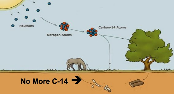
Of all the elements, carbon is the one that seems most indispensable to life – the one without which life on any planet is hardest to envisage. This is because of carbon’s remarkable capacity for forming chains and rings and other complex molecular architectures. It enters the food web via photosynthesis, which is the process whereby green plants take in carbon dioxide molecules from the atmosphere and use energy from sunlight to combine the carbon atoms with water to make sugars. All the carbon in ourselves and in all other living creatures comes ultimately, via plants, from carbon dioxide in the atmosphere. And it is continually being recycled back to the atmosphere: when we breathe out, when we excrete, and when we die.
Most of the carbon in the atmosphere’s carbon dioxide is carbon-12, which is not radioactive. However, about one atom in a trillion is carbon-14, which is radioactive. It decays rather rapidly, with a half-life of 5,730 years, as we have seen, to nitrogen-14. Plant biochemistry is blind to the difference between these two carbons. To a plant, carbon is carbon is carbon. So plants take in carbon-14 alongside carbon-12, and incorporate the two kinds of carbon atom in sugars, in the same proportion as they exist in the atmosphere. The carbon that is incorporated from the atmosphere (complete with the same proportion of carbon-14 atoms) is rapidly (compared to the half-life of carbon-14) spread through the food chain, as plants are eaten by herbivores, herbivores by carnivores and so on. All living creatures, whether plants or animals, have approximately the same ratio of carbon-12 to carbon-14, which is the same ratio as you’ll find in the atmosphere.
So, when is the clock zeroed? At the moment when a living creature, whether animal or plant, dies. At that moment, it is severed from the food chain, and detached from the inflow of fresh carbon-14, via plants, from the atmosphere. As the centuries go by, the carbon-14 in the corpse, or lump of wood, or piece of cloth, or whatever it is, steadily decays to nitrogen-14. The ratio of carbon-14 to carbon-12 in the specimen therefore gradually drops further and further below the standard ratio that living creatures share with the atmosphere. Eventually it will be all carbon-12 – or, more strictly, the carbon-14 content will become too small to measure. And the ratio of carbon-12 to carbon-14 can be used to calculate the time that has elapsed since the death of the creature cut it off from the food chain and its interchange with the atmosphere.
Carbon-14 is special because it is continually being made by cosmic rays bombarding nitrogen atoms in the upper atmosphere. Nitrogen is the commonest gas in the atmosphere and its mass number is 14, the same as carbon-14’s. The difference is that carbon-14 has 6 protons and 8 neutrons, while nitrogen-14 has 7 protons and 7 neutrons (neutrons, remember, have near-enough the same mass as protons). Cosmic ray particles are capable of hitting a proton in a nitrogen nucleus and converting it to a neutron. When this happens, the atom becomes carbon-14, carbon being one lower than nitrogen in the periodic table. The rate at which this conversion occurs is approximately constant from century to century, which is why carbon dating works.
Carbon dating is a comparatively recent invention, going back only to the 1940s. In its early years, substantial quantities of organic material were needed for the dating procedure. Then, in the 1970s, a technique called mass spectrometry was adapted to carbon dating, with the result that only a tiny quantity of organic material is now needed. This has revolutionized archaeological dating. The most celebrated example is the Shroud of Turin. Since this notorious piece of cloth seems mysteriously to have imprinted on it the image of a bearded, crucified man, many people hoped it might hail from the time of Jesus. It first turns up in the historical record in the mid-fourteenth century in France, and nobody knows where it was before that. It has been housed in Turin since 1578, under the custody of the Vatican since 1983. When mass spectrometry made it possible to date a tiny sample of the shroud, rather than the substantial swathes that would have been needed before, the Vatican allowed a small strip to be cut off. The strip was divided into three parts and sent to three leading laboratories specializing in carbon dating, in Oxford, Arizona and Zurich. Working under conditions of scrupulous independence – not comparing notes – the three laboratories reported their verdicts on the date when the flax from which the cloth had been woven died. Oxford said ad 1200, Arizona 1304 and Zurich 1274.
Radioactive clocks can be used to give independent estimates of the age of one piece of rock, bearing in mind that all the clocks were zeroed simultaneously when this very same piece of rock solidified. When such comparisons have been made, the different clocks agree with each other – within the expected margins of error. This gives great confidence in the correctness of the clocks. Thus mutually calibrated and verified on known rocks, these clocks can be carried with confidence to interesting dating problems, such as the age of the Earth itself. The currently agreed age of 4.6 billion years is the estimate upon which several different clocks converge.
Before our eyes
Although the vast majority of evolutionary change took place before any human being was born, some examples are so fast that we can see evolution happening with our own eyes during one human lifetime.
There’s a plausible indication that this may have happened even with elephants, which Darwin himself picked out as one of the slowest-reproducing animals, with one of the longest generation turnovers. One of the main causes of mortality among African elephants is humans with guns hunting ivory, either for trophies or to sell for carving. Naturally the hunters tend to pick on the individuals with the largest tusks. This means that, at least in theory, smaller-tusked individuals will be at a selective advantage. As ever with evolution, there will be conflicting selection pressures, and what we see evolving will be a compromise. Larger tuskers doubtless have an advantage when it comes to competition with other elephants, and this will be balanced against their disadvantage when they encounter men with guns. Any increase in hunting activity, whether in the form of illegal poaching or legal hunting, will tend to shift the balance of advantage towards smaller tusks. All other things being equal, we might expect an evolutionary trend towards smaller tusks as a result of human hunting, but we’d probably expect it to take millennia to be detectable. We would not expect to see it within one human lifetime. Now let’s look at some figures.
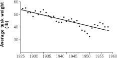
Fig. Tusk weight in Ugandan elephants
The graph above shows data from the Uganda Game Department, published in 1962. Referring only to elephants legally shot by licensed hunters, it shows mean tusk weight in pounds (that dates it) from year to year between 1925 and 1958 (during which time Uganda was a British protectorate). The dots are annual figures. You can see that there is a decreasing trend over the thirty-three years. And the trend is highly statistically significant, which means that it is almost certainly a real trend, not a random chance effect.
The lizards of Pod Mrcaru
There are two small islets off the Croatian coast called Pod Kopiste and Pod Mrcaru. In 1971 a population of common Mediterranean lizards, Podarcis sicula, which mainly eat insects, was present on Pod Kopiste but there were none on Pod Mrcaru. In that year experimenters transported five pairs of Podarcis sicula from Pod Kopiste and released them on Pod Mrcaru. Then, in 2008, another group of mainly Belgian scientists, associated with Anthony Herrel, visited the islands to see what had happened. They found a flourishing population of lizards on Pod Mrcaru, which DNA analysis confirmed were indeed Podarcis sicula. These are presumed to have descended from the original five pairs that were transported. Herrel and his colleagues made observations on the descendants of the transported lizards, and compared them with lizards living on the original ancestral island. There were marked differences.
The Pod Mrcaru lizards – the ‘evolved’ population – had significantly larger heads than the ‘original’ Pod Kopiste population: longer, wider and taller heads. This translates into a markedly greater bite force. A change of this kind typically goes with a shift to a more vegetarian diet. Herbivorous mammals like horses, cattle and elephants have great millstone-like teeth for grinding cellulose of plants, quite different from the shearing teeth of carnivores and the needly teeth of insectivores. This experiment shows that in exceptional condtions evolution can happen extremely rapidly, in a matter of a few decades: evolution before our very eyes.
 Forty five thousand generations of evolution in a lab
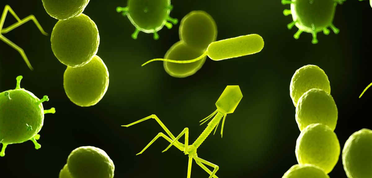
The average generation turnover of those lizards is about two years, so the evolutionary change observed on Pod Mrcaru represents only about eighteen or nineteen generations. Just think what you might see in three or four decades if you followed the evolution of bacteria, whose generations are measured in hours or even minutes, rather than years! Bacteria offer another priceless gift to the evolutionist. In some cases you can freeze them for an indefinite length of time and then bring them back to life again, whereupon they resume reproduction as if nothing had happened. This means that experimenters can lay down their own ‘living fossil record’, a snapshot of the exact point the evolutionary process had reached at any desired time.
E. coli is a common bacterium. Very common. There are about a hundred billion billion of them around the world at any one time, of which about a billion, by Lenski’s calculation, are in your large intestine at this very moment. If we assume that the probability of a gene mutating during any one act of bacterial reproduction is as low as one in a billion, the numbers of bacteria are so colossal that just about every gene in the genome will have mutated somewhere in the world, every day. As Richard Lenski says, ‘That’s a lot of opportunity for evolution.’
These bacteria reproduce asexually – by simple cell division – so it is easy to clone up a huge population of genetically identical individuals in a short time. In 1988, Lenski took one such population and infected twelve identical flasks, all of which contained the same nutrient broth, including glucose as the vital food source. These twelve flasks founded twelve lines of evolution that were destined to be kept separate from one another for two decades and counting: sort of like the twelve tribes of Israel, except that in the case of the tribes of Israel there was no law against their mixing.
Every day, for each of the twelve tribes, a new virgin flask was infected with liquid from the previous day’s flask. A small sample, exactly one-hundredth of the volume of the old flask, was drawn out and squirted into the new flask, which contained a fresh supply of glucose-rich broth. The population of bacteria in the flask then started to skyrocket; but it always levelled off by the next day as the supply of food gave out and starvation set in. In other words, the population in every flask multiplied itself hugely, then reached a plateau, at which point a new infective sample was drawn and the cycle renewed the next day.
Lenski and his team have continued this daily routine for more than twenty years so far. This means about 7,000 ‘flask generations’ and 45,000 bacterial generations – averaging between six and seven bacterial generations per day. To put that into perspective, if we were to go back 45,000 human generations, that would be about a million years, back to the time of Homo erectus, which is not very long ago.
The Lenski lab had earlier exploited a gene called ara which comes in two forms, Ara+ and Ara−. You can’t tell the difference until you take a sample of the bacteria and ‘plate them out’ on an agar plate that contains a nutritious broth plus the sugar arabinose and a chemical dye called tetrazolium. ‘Plating out’ is one of the things bacteriologists do. It means putting a drop of liquid, containing bacteria, on a plate covered with a thin sheet of agar gel and then incubating the plate. Colonies of bacteria grow out as expanding circles – miniature fairy rings – from the drops, feeding on the nutrients mixed in with the agar. If the mixture contains arabinose and the indicator dye, the difference between Ara+ and Ara− is revealed, as if by heating invisible ink: they show up as white and red colonies, respectively. The Lenski team settles up six of their twelve tribes as Ara+ and the other six as Ara−.
The broth, as I have said, contained glucose. It was not the only food there, but it was the limiting resource. This means that running out of glucose was the key factor that caused the population size, in every flask every day, to stop climbing and reach a plateau. In these conditions, the Darwinian expectation was that, if any mutation arose that assisted an individual bacterium to exploit glucose more efficiently, natural selection would favour it, and it would spread through the flask as mutant individuals out-reproduced non-mutant individuals. Its type would then disproportionately infect the next flask in the lineage and, as flask took over from flask, pretty soon the mutant would have a monopoly of its tribe. Well, this is exactly what happened in all twelve tribes. As the ‘flask generations’ went by, all twelve lines improved over their ancestors: got better at exploiting glucose as a food source. But, fascinatingly, they got better in different ways – that is, different tribes developed different sets of mutations.
How did the scientists know this? They could tell by sampling the lineages as they evolved, and comparing the ‘fitness’ of each sample against ‘fossils’ sampled from the original founding population. Remember that ‘fossils’ are frozen samples of bacteria which, when unfrozen, carry on living and reproducing normally. And how did Lenski and his colleagues make this comparison of ‘fitness’? How did they compare ‘modern’ bacteria with their ‘fossil’ ancestors? With great ingenuity. They took a sample of the putatively evolved population and put it in a virgin flask.
We have a new experimental flask containing two competing strains, ‘modern’ and ‘living fossil’, and we want to know which of the two strains will out-populate the other. But they are all mixed up, so how do you tell? How do you distinguish the two strains, when they are mixed together in the ‘competition flask’? They could use the colour markers to assay the competitive abilities of each of the evolving tribes, using fossilized ‘ancestors’ as the competitive standard, in every case. All they had to do was simply plate out samples from the mixed flasks and see how many of the bacteria growing on the agar were white and how many red. In all twelve tribes the average fitness increased as the thousands of generations went by. All twelve lines got better at surviving in these glucose-limited conditions.
What this evolutionary change suggests is that becoming larger is, for some reason, a good idea when you are struggling to survive in this alternating glucose-rich/glucose-poor environment. But there are lots of different ways to become larger – different sets of mutations – and it looks as though different ways have been discovered by different evolutionary lineages in this experiment. That’s pretty interesting. But perhaps even more interesting is that sometimes a pair of tribes seem to have independently discovered the same way of getting bigger. Lenski and a different set of colleagues investigated this phenomenon by taking two of the tribes, called Ara+1 and Ara−1, which seemed, over 20,000 generations, to have followed the same evolutionary trajectory, and looking at their DNA. The astonishing result they found was that 59 genes had changed their levels of expression in both tribes, and all 59 had changed in the same direction.
The data are at least compatible with the idea that the evolutionary change that we observe represents the stepwise accumulation of mutations.
So far, I’ve implied that all twelve tribes evolved their improved fitness in the same general kind of way, differing only in detail – some being a bit faster, some a bit slower than others. However, the long-term experiment threw up one dramatic exception. Shortly after generation 33,000 something utterly remarkable happened. One out of the twelve lineages, called Ara−3, suddenly went berserk.
Up to about generation 33,000, the average population density of Tribe Ara−3 was coasting along at an OD of about 0.04, which was not very different from all the other tribes. Then, just after generation 33,100, the OD score of Tribe Ara−3 (and of that tribe alone among the twelve) went into vertical take-off. It shot up sixfold, to an OD value of about 0.25.
What was going on? What was it that suddenly happened to Tribe Ara−3? Lenski and two colleagues investigated further, and worked it out. It is a fascinating story. You remember I said that glucose was the limiting resource, and any mutant that ‘discovered’ how to deal more efficiently with glucose would have an advantage. That indeed is what happened in the evolution of all twelve tribes. But I also told you that glucose was not the only nutrient in the broth. Another one was citrate (related to the substance that makes lemons sour). The broth contained plenty of citrate, but E. coli normally can’t use it, at least not where there is oxygen in the water, as there was in Lenski’s flasks. But if only a mutant could ‘discover’ how to deal with citrate, a bonanza would open up for it. This is exactly what happened with Ara−3. This tribe, and this tribe alone, suddenly acquired the ability to eat citrate as well as glucose, rather than only glucose.
Having discovered what was special about the Ara−3 tribe, Lenski and his colleagues went on to ask an even more interesting question. Was this sudden improvement in ability to draw nourishment all due to a single dramatic mutation, one so rare that only one of the twelve lineages was fortunate enough to undergo it?
This seemed to Lenski unlikely, for an interesting reason. Knowing the average mutation rate of each gene in the genome of these bacteria, he calculated that 30,000 generations was long enough for every gene to have mutated at least once in each of the twelve lines. So it seemed unlikely that it was the rarity of the mutation that singled Ara−3 out. It should have been ‘discovered’ by several other tribes.
What if the necessary biochemical wizardry to feed on citrate requires not just one mutation but two (or three)? On this hypothesis, you really would need both mutations before there is any improvement whatsoever. The hypothesis, is that, at some time unknown, Tribe Ara−3 chanced to undergo a mutation, mutation A. This had no detectable effect because the other necessary mutation, B, was still lacking. Mutation B is equally likely to crop up in any one of the twelve tribes. Indeed, it probably did. But B is no use – has absolutely no beneficial effect at all – unless the tribe happens to be primed by the previous occurrence of mutation A. And only tribe Ara−3, as it happened, was so primed.
"Some of these Lazarus clones will ‘discover’ how to deal with citrate, but only if they were thawed out of the fossil record after a particular, critical generation in the original evolution experiment."-Lenski
You will be delighted to hear that this is exactly what Lenski’s student Zachary Blount found, when he ran a gruelling set of experiments involving some forty trillion – 40,000,000,000,000 – E. coli cells from across the generations. The magic moment turned out to be approximately generation 20,000. Thawed- out clones of Ara−3 that dated from after generation 20,000 in the ‘fossil record’ showed increased probability of subsequently evolving citrate capability. No clones that dated from before generation 20,000 did. According to the hypothesis, after generation 20,000 the clones were now ‘primed’ to take advantage of mutation B whenever it came along. Tribe Ara−3, before generation 20,000, was just like all the other tribes.
Guppies
Guppies are popular freshwater aquarium fish. As the pheasants, the males are more brightly coloured than the females, and aquarists have bred them to become even brighter. In some populations the adult males are rainbow-coloured, almost as bright as those bred in aquarium tanks. He surmised that their ancestors had been selected for their bright colours by female guppies, in the same manner as cock pheasants are selected by hens. In other areas the males were much drabber, although they were still brighter than the females. Like the females, though less so, they were well camouflaged against the gravelly bottoms of the streams in which they live. The pressure from females on males to evolve bright colours was there all the time, in all the various separate populations, whether the local predators were pushing in the other direction strongly or weakly. As ever, evolution finds a compromise between selection pressures.
So, here’s the set-up: guppies were assigned randomly to ten ponds, five with coarse gravel and five with fine gravel. All ten colonies of guppies were allowed to breed freely for six months with no predators. At this point the experiment proper began. Endler put one ‘dangerous predator’ into each of two coarse gravel ponds and two fine gravel ponds. He put six ‘weak predators’ (six rather than one, to give a closer approximation to the relative densities of the two kinds of fish in the wild) into each of two coarse gravel ponds and two fine gravel ponds. And the remaining two ponds just carried on as before, with no predators at all.
After the experiment had been running for five months, Endler took a census of all the ponds, and counted and measured the spots on all the guppies in all the ponds. Nine months later, that is, after fourteen months in all, he took another census, counting and measuring in the same way. And what of the results? They were spectacular, even after so short a time. Endler used various measures of the fishes’ colour patterns, one of which was ‘spots per fish’. When the guppies were first put into their ponds, before the predators were introduced, there was a very large range of spot numbers, because the fish had been gathered from a wide variety of streams, of widely varying predator content. During the six months before any predators were introduced, the mean number of spots per fish shot up. Presumably this was in response to selection by females. Then, at the point when the predators were introduced, there was a dramatic change. In the four ponds that had the dangerous predator, the mean number of spots plummeted. The difference was fully apparent at the five-month census, and the number of spots had declined even further by the fourteen-month census. But in the two ponds with no predators, and the four ponds with weak predation, the number of spots continued to increase. It reached a plateau as early as the five-month census, and stayed high for the fourteen-month census. With respect to spot number, weak predation seems to be pretty much the same as no predation, over-ruled by sexual selection by females who prefer lots of spots.
So much for spot number. Spot size tells an equally interesting story. In the presence of predators, whether weak or strong, coarse gravel promoted relatively larger spots, while fine gravel favoured relatively smaller spots. This is easily interpreted as spot size mimicking stone size. Fascinatingly, however, in the ponds where there were no predators at all, Endler found exactly the reverse. Fine gravel favoured large spots on male guppies, and coarse gravel favoured small spots. They are more conspicuous if they do not mimic the stones on their respective backgrounds, and that is good for attracting females. Neat!
 Missing link
The biggest gap, and the one the creationists like best of all, is the one that preceded the so-called Cambrian Explosion. A little more than half a billion years ago, in the Cambrian era, most of the great animal phyla – the main divisions within the animal world – ‘suddenly’ appear in the fossil record. Suddenly, that is, in the sense that no fossils of these animal groups are known in rocks older than the Cambrian, not suddenly in the sense of instantaneously: the period we are talking about covers about 20 million years. Twenty million years feels short when it is half a billion years ago.
There are more than four thousand species of free-living turbellarian worms : that’s about as numerous as all the mammal species put together. Some of these turbellarians are creatures of great beauty. They are common, both in water and on land, and presumably have been common for a very long time. You’d expect, therefore, to see a rich fossil history. Unfortunately, there is almost nothing. Apart from a handful of ambiguous trace fossils, not a single fossil flatworm has ever been found. The Platyhelminthes, to a worm, are ‘already in an advanced state of evolution, the very first time they appear. It is as though they were just planted there, without any evolutionary history.’
Probably, most animals before the Cambrian were soft-bodied like modern flatworms, probably also rather small like modern turbellarians – just not good fossil material. Then something happened half a billion years ago to allow animals to fossilize freely – the arising of hard, mineralized skeletons, for example.
Show me your crocoduck
Hippopotamuses do not descended from dogs, or vice versa. Chimpanzees are not descended from elephants or vice versa, just as monkeys are not descended from frogs. No modern species is descended from any other modern species (if we leave out very recent splits). Just as you can find fossils that approximate to the common ancestor of a frog and a monkey, so you can find fossils that approximate to the common ancestor of elephants and chimpanzees.
The pernicious legacy of the great chain of being
Zoologists have traditionally divided the vertebrates into classes: major divisions with names like mammals, birds, reptiles and amphibians. Some zoologists, called ‘cladists’,* insist that a proper class must consist of animals all of whom share a common ancestor which belonged to that class and which has no descendants outside that group. The birds would be an example of a good class.† All birds are descended from a single ancestor that would also have been called a bird and would have shared with modern birds the key diagnostic characters – feathers, wings, a beak, etc. The animals commonly called reptiles are not a good class in this sense. This is because, at least in conventional taxonomies, the category explicitly excludes birds (they constitute their own class) and yet some ‘reptiles’ as conventionally recognized (e.g. crocodiles and dinosaurs) are closer cousins to birds than they are to other ‘reptiles’ (e.g. lizards and turtles). Indeed, some dinosaurs are closer cousins to birds than they are to other dinosaurs. ‘Reptiles’, then, is an artificial class, because birds are artificially excluded. In a strict sense, if we were to make reptiles a truly natural class, we should have to include birds as reptiles. Cladistically inclined zoologists avoid the word ‘reptiles’ altogether, splitting them into Archosaurs (crocodiles, dinosaurs and birds), Lepidosaurs (snakes, lizards and the rare Sphenodon of New Zealand) and Testudines (turtles and tortoises).
The closest relatives of birds are all to be found among the longextinct dinosaurs. If the cards of extinction had fallen differently, there would just be lots of dinosaurs running about, including some feathered, flying, beaked dinosaurs called birds. And indeed, fossilized feathered dinosaurs are now increasingly being discovered.
Up from the sea
Short of rocketing into space, it is hard to imagine a bolder or more life-changing step than leaving the water for dry land. The two life-zones are different in so many ways that moving from one to the other demands a radical shift in almost all parts of the body. Gills that are good at extracting oxygen from water are all but useless in air, and lungs are useless in water. Methods of propulsion that are speedy, graceful and efficient in water are dangerously clumsy on land, and vice versa.
Fish are defined by exclusion. Fish are all the vertebrates except those that moved on to the land. Trout and tuna are closer cousins to humans than they are to sharks, but we call them all ‘fish’. Vertebrates whose ancestors never ventured on to land all look like ‘fish’, they all swim like fish (unlike dolphins, which swim with an up-and-down bending of the spine instead of side to side like a fish), and they all, I suspect, taste like fish.
If we then push to one side the bony ‘ray-finned fishes’ (salmon, trout, tuna, angel fish: just about all the fish you are likely to see that are not sharks), the natural group to which we belong includes all land vertebrates plus the so-called lobe-finned fishes. It is from the ranks of the lobe-finned fishes that we sprang, and we must now pay special attention to the lobefins.
Go down to the sea again
The move from water to land launched a major redesign of every aspect of life, from breathing to reproduction: it was a great trek through biological space. Nevertheless,
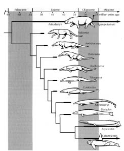
with what seems almost wanton perversity, a good number of thoroughgoing land animals later turned around, abandoned their hard- earned terrestrial retooling, and trooped back into the water again. Seals and sea lions have only gone part-way back. They show us what the intermediates might have been like, on the way to extreme cases such as whales and dugongs. Whales (including the small whales we call dolphins), and dugongs with their close cousins the manatees, ceased to be land creatures altogether and reverted to the full marine habits of their remote ancestors. They don’t even come ashore to breed. They do, however, still breathe air, having never developed anything equivalent to the gills of their earlier marine progenitors.
Whales were long an enigma, but recently our knowledge of whale evolution has become rather rich. Molecular genetic evidence shows that the closest living cousins of whales are hippos, then pigs, then ruminants. Even more surprisingly, the molecular evidence shows that hippos are more closely related to whales than they are to the cloven-hoofed animals (such as pigs and ruminants) which look much more like them. Hippos stayed, at least partly, on land, and so still resemble their more distant land-dwelling cousins, the ruminants, while their closer cousins, the whales, took off into the sea and changed so drastically that their affinities with hippos escaped all biologists except molecular geneticists.
the turtles accomplished an evolutionary doubling back to the land: an early marque of land ‘tortoises’ went back to the watery environment of their even earlier fish ancestors, became sea turtles, then returned to the land yet again, as a new incarnation of land tortoises, the Testudinidae.
Missing Persons
I am still mischievously hoping
The most famous fossil of this vintage is ‘Lucy’, classified by her discoverer in Ethiopia, Donald Johanson, as Australopithecus afarensis. Lucy’s skeleton is complete enough to suggest that she walked upright on the ground, but probably also sought refuge in trees, where she was an agile climber. The conclusion from studies of Lucy and her kind is that they had brains about the same size as chimpanzees’ but, unlike chimpanzees, they walked upright on their hind legs, as we do. What matters is that, by 3.6 million years ago, an erect ape walked the Earth, on two feet which were pretty much like ours although its brain was the size of a chimpanzee’s.
Genus is the more inclusive division. A species belongs within a genus, and often it shares the genus with other species. Homo sapiens and Homo erectus are two species within the genus Homo.
You did it your self in nine months
 No choreographer
An architect designs a great cathedral. Then, through a hierarchical chain of command, the building operation is broken down into separate departments, which break it down further into sub-departments, and so on until instructions are finally handed out to individual masons, carpenters and glaziers, who go to work until the cathedral is built, looking pretty much like the architect’s original drawing. That’s top- down design.
Bottom-up design works completely differently. I never believed this, but there used to be a myth that some of the finest medieval cathedrals in Europe had no architect. Nobody designed the cathedral. Each mason and carpenter would busy himself, in his own skilled way, with his own little corner of the building, paying scant attention to what the others were doing and no attention to any overall plan. Somehow, out of such anarchy, a cathedral would emerge. If that really happened, it would be bottom-up architecture. Notwithstanding the myth, it surely didn’t happen like that for cathedrals.* But that pretty much is what happens in the building of a termite mound or an ant’s nest – and in the development of an embryo. It is what makes embryology so remarkably different from anything we humans are familiar with, in the way of construction or manufacture.
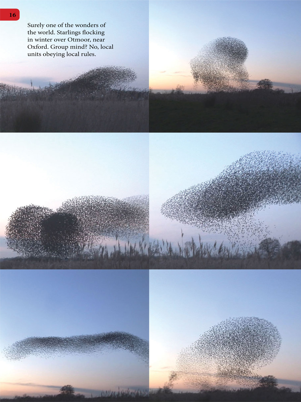
Suppose we wanted to understand the flocking behaviour of starlings. What is remarkable about the starlings’ behaviour is that, despite all appearances, there is no choreographer and, as far as we know, no leader. Each individual bird is just following local rules. The numbers of individual birds in these flocks can run into thousands, yet they almost literally never collide.
Here’s how to program flocking behaviour in starlings. Devote almost all your effort to programming the behaviour of a single individual bird. Build into your robo-starling detailed rules for how to fly, and how to react to the presence of neighbouring starlings, depending on their distance and relative position. Build in rules for how much weight to give to the behaviour of neighbours, and how much weight to give to individual initiative in changing direction. These model rules would be informed by careful measurements of real birds in action. Endow your cyberbird with a certain tendency to vary its rules at random. Having written a complicated program to specify the behavioural rules of a single starling, now comes the definitive step that I am emphasizing in this chapter. Don’t try to program the behaviour of a whole flock, as an earlier generation of computer programmers might have done. Instead, clone the single computer starling you have programmed. Make a thousand copies of your robo-bird, maybe all the same as each other, or maybe with some slight random variation among them in their rules. And now ‘release’ thousands of model starlings in your computer, so they are free to interact with each other, all obeying the same rules.
The key point is that there is no choreographer and no leader. Order, organization, structure – these all emerge as by-products of rules which are obeyed locally and many times over, not globally. And that is how embryology works. It is all done by local rules, at various levels but especially the level of the single cell. No choreographer. No conductor of the orchestra.
Analogies for development
Unlike a blueprint, a recipe is irreversible. If you follow a cake recipe step by step, you’ll end up with a cake. But you can’t take a cake and reconstruct the recipe – certainly not the exact words of the recipe – whereas, as we have seen, you could take a house and reconstruct something close to the original blueprint. This is because of the one- to-one mapping between bits of house and bits of blueprint.
Enzymes
Proteins are chains of smaller molecules called amino acids, and these chains, like the sheets of cells we have been considering, also fold themselves, in highly determined ways but on a much smaller scale. In naturally occurring proteins (this is one fact that will presumably be different on alien worlds) there are only twenty kinds of amino acid, and all proteins are chains strung together from just this repertoire of twenty, drawn from a much larger set of possible amino acids. Now for the auto-origami. Protein molecules, simply following the laws of chemistry and thermodynamics, spontaneously and automatically twist themselves into precisely shaped three-dimensional configurations – I almost said ‘knots’ but, unlike hagfish (if I might impart a gratuitously inconsequential but engaging fact), proteins don’t literally tie themselves in knots. The three-dimensional structure into which a protein chain folds and twists itself is the ‘tertiary structure’ that we briefly met when considering the self-assembly of viruses. Any given sequence of amino acids dictates a particular folding pattern. The amino-acid sequence, which itself is determined by the sequence of letters in the genetic code, determines the shape of the tertiary pattern.* The shape of the tertiary structure, in turn, has hugely important chemical consequences.
Even though it is not easy for human chemists to predict what change in protein shape will result from a particular genetic mutation, it is still a fact that once a mutation has occurred, the resulting change of protein shape will be in principle predictable. The same mutant gene will reliably produce the same altered protein shape (or discrete menu of alternative shapes). And that is all that matters for natural selection. Natural selection doesn’t need to understand why a genetic change has a certain consequence. It is sufficient that it does. If that consequence affects survival, the changed gene itself will stand or fall in the competition to dominate the gene pool, whether or not we understand the exact route by which the gene affects the protein.
The point of this section of the chapter is that ‘the right enzyme’ achieves its ‘rightness’ largely through its physical shape (and that’s important, because the physical shape is determined by genes, and it is genes whose variations are ultimately favoured or disfavoured by natural selection). Molecules aplenty are drifting and twisting and spinning through the soup that bathes the interior of a cell. A molecule of substance A might be happy to react with a molecule of substance B, but only if they happen to collide when facing in exactly the right direction, relative to each other. Crucially, that seldom happens – unless the right enzyme intervenes. The enzyme’s precise shape, the shape into which it folded itself like a magnetic necklace, leaves it pitted with cavities and dents, each one of which itself has a precise shape. Each enzyme has a so-called ‘active site’, which is usually a particular dent or pocket, whose shape and chemical properties confer upon the enzyme its specificity.
Every cell, with very few exceptions such as red blood corpuscles, which lack a nucleus, contains the genes for making all the enzymes. But in any one cell, only a few genes will be turned on at any one time. It is genes which determine sequences of amino acids, which determine tertiary structures of proteins, which determine the socket-like shapes of active sites, which determine cell chemistry, which determine ‘starling-like’ cell behaviour in embryonic development. So, differences in genes can, at the originating end of the complex chain of events, cause differences in the way embryos develop, and hence differences in the form and behaviour of adults. The survival and reproductive success of those adults then feeds back on the survival in the gene pool of the genes that made the difference between success and failure. And that is natural selection.
Then worms shall try
Whether or not a given gene is turned on in a given cell at a given time is determined, often via a cascade of other genes called switch genes or controller genes, by the chemical environment of the cell.
We now know everything about Caenorhabditis elegans! We know its entire genome. We know exactly where every one of its 558 cells (in the larva; 959 in the adult hermaphroditic form, not counting reproductive cells) is in the body, and we know the exact ‘family history’ of every one of those cells, through embryonic development.
The number of cell ‘generations’ that separates the tissues from the original egg is not that great. After all, there are only 558 cells in the body, and you can theoretically make 1,024 (2 to the power 10) in ten generations of cell splitting. The numbers of cell generations for human cells would be much larger. Nevertheless, you could in theory make a similar family tree for every one of your trillion-odd cells (as opposed to the 558 cells of a C. elegans female larva), tracing each one’s descent back to the one fertilized egg cell.
when the cell divided, the two daughter cells, though identical in their genes (every daughter cell receives a full complement of genes), were not identical in the surrounding chemicals. And this meant that the same genes were not turned on – which changed the fate of their descendants. The same principle applies right through embryology, including its very start. The key to differentiation, in all animals, is asymmetric cell division. In Caenorhabditis the original cell, called Z, has a front end which is different from its rear end, and this difference will come to represent the eventual fore-and-aft body axis – anterior (front) and posterior (rear). When the cell divides, the anterior daughter cell, which is called AB, has more front-end substance than the posterior daughter cell, which is called P1, and this difference will be bootstrapped to make more differences down the line.
Sir John Sulston and his colleagues traced each of the cells in the body of the worm back to one and only one of six founder cells – we might even call them ‘matriarch’ cells – called AB, MS, E, D, C and P4. In naming the cells, they used a neat notation that summarized the history of each one. Every cell’s name begins with the name of one of those six founder cells, the one from which it is descended. Thereafter, its name is a string of letters, the initial letters of the direction of cell division that gave rise to it: anterior, posterior, dorsal, ventral, left, right. For example, Ca and Cp are the two daughters of matriarch C, the anterior and posterior daughter respectively. ABprpapppap, to take another example, is a nerve cell that sits in the ventral nerve cord running along the length of the worm. Every one of the ten cell divisions that gave rise to ABprpapppap, and every other cell, was an asymmetric division with the potential for different genes to be switched on in each of the two daughter cells. In any animal, cells differ from each other in different parts of the body, even though they are genetically identical, because of their history of asymmetric cell division during the short course of embryonic development.
The development of the embryo, and ultimately of the adult, is achieved by local rules implemented by cells, interacting with other cells on a local basis. What goes on inside cells, similarly, is governed by local rules that apply to molecules, especially protein molecules, within the cells and in the cell membranes, interacting with other such molecules. Again, the rules are all local, local, local. Nobody, reading the sequence of letters in the DNA of a fertilized egg, could predict the shape of the animal it is going to grow into. The only way to discover that is to grow the egg, in the natural way, and see what it turns into.
The ark of the continents
How new species are born
Every species is a cousin of every other. Any two species are descended from an ancestral species, which split in two. For example, the common ancestor of people and budgerigars lived about 310 million years ago. In the unlikely event that a fossil of these ancestral species was ever found, it would need a name. Let’s call it Protamnio darwinii. When Protamnio darwinii split into two sub-populations they would have looked just the same as each other, and could have happily interbred with each other; but one lot were destined to give rise to the mammals, and the other lot were destined to give rise to the birds (and dinosaurs and snakes and crocodiles). These two sub-populations of Protamnio darwinii were about to diverge from each other, over a very long time and in a very big way. But they couldn’t diverge if they kept on interbreeding with each other. The two gene pools would continually flood each other with genes. So any tendency to diverge would be nipped in the bud before it could get going, swamped by gene flow from the other population.
The two sub-populations of Protamnio darwinii somehow became separated from each other, most likely by a geographical barrier such as a strip of sea separating two islands, or separating an island from a mainland. It could have been a mountain range that separated two valleys, or a river separating two forests: two ‘islands’ in the general sense I defined. All that matters is that the two populations were isolated from one another for long enough so that, when time and chance eventually reunited them, they found they had diverged so much that they couldn’t interbreed any more.
Even if conditions on either side of the barrier are identical, two geographically separated gene pools of the same species will eventually drift apart from one another, to the point where they can no longer interbreed when the geographical isolation eventually comes to an end. Random changes in the two gene pools will gradually build up, to the point where, if a male and a female from the two sides meet, their genomes will be too different to combine to make a fertile offspring.
One might really fancy
How, then, do two populations of a species find themselves on opposite sides of a geographical barrier? Sometimes the barrier itself is the novelty. An earthquake opens up an impassable gorge, or changes the course of a river, and a species that had been a single breeding population finds itself severed in two. More usually, the barrier was there all along, and it is the animals themselves that cross it, in a rare freak event. It has to be rare, otherwise it doesn’t deserve to be called a barrier at all.
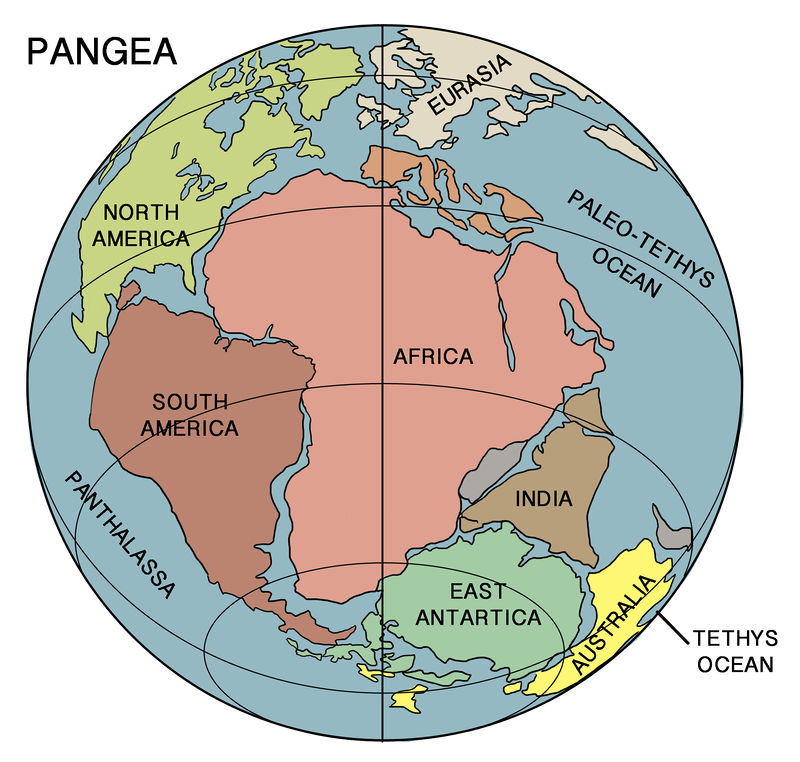
Did the Earth move ?
The theory of ‘continental drift’, as it used to be called, was first championed by the German climatologist Alfred Wegener (1880–1930). Wegener was not the first to look at a map of the world and notice that the shape of a continent or island often matches the coastline opposite as if the two land masses were pieces of a jigsaw puzzle, even when the opposite coastline is far away. I’m not talking about little local examples, such as the Isle of Wight’s neat dovetailing into the Hampshire coast, almost as though the Solent wasn’t there. What Wegener and his predecessors noticed was that something along the same lines seemed to be true of the whole facing sides of the giant continents of Africa and America. The Braz
ilian coast looks tailor-cut to fit under the bulge of West Africa, while the northern part of Africa’s bulge is a nice fit to the North American coast from Florida to Canada. Not only do the shapes roughly match: Wegener also pointed to matching geological formations up and down the east side of South America and corresponding parts of the west side of Africa. Slightly less clearly, the west coast of Madagascar forms a pretty good fit to the east coast of Africa (not the section of South African coast that is opposite it today but the coast of Tanzania and Kenya further north), while the long, straight
line of Madagascar’s east side is comparable to the straight edge of western India. Wegener also pointed out that the ancient fossils to be found in Africa and South America were more similar than you would expect if the map of the world had always been the way it is today. How could this be, given the width of the South Atlantic ocean? Were the two continents once much closer, or even joined? The idea was tantalizing, but ahead of its time. Wegener also noticed matchings between the fossils of Madagascar and India. And there are similarly telling affinities between the fossils of northern North America and of Europe.
Such observations led Wegener to propose his daringly heretical hypothesis of continental drift. All the great continents of the world, he suggested, had once been joined up in a gigantic super-continent, which he called Pangaea. Over an immense span of geological time, he proposed, Pangaea gradually dismembered itself to form the continents we know today, which then slowly drifted to their present positions and have not finished drifting yet.
In the theory of plate tectonics the whole of the Earth’s surface, including the bottoms of the various oceans, consists of a series of overlapping rocky plates like a suit of armour. The continents that we see are thickenings of the plates that rise above sea level. The greater part of the area of each plate lies under the sea. Unlike Wegener’s continents, the plates do not sail through the sea, or plough through the surface of the Earth, they are the surface of the Earth.
South America and Africa, and their continental shelves, are but the thickened regions of two plates, much of whose rocky surfaces lies under the sea. The plates constitute the hard lithosphere – literally, ‘sphere of rock’ – which floats atop the hot, semi-molten asthenosphere – ‘sphere of weakness’.
Madagascar and Africa were once part of the great southern continent of Gondwana, together with South America, Antarctica, India and Australia. Gondwana began to break up – painfully slowly by the standards of our perception – about 165 million years ago. At this point Madagascar, while still joined to India, Australia and Antarctica as East Gondwana, pulled away from the eastern side of Africa. At about the same time, South America pulled away from West Africa in the other direction. East Gondwana itself broke up rather later, and Madagascar finally became separated from India about 90 million years ago.
The tree of cousinship
 Bone to his bone
The skeletons of all mammals are identical, but their individual bones are different. ‘Skeleton’, in this special sense, ignores the shapes of individual bones, and is concerned only with the order in which they join up: ‘bone to his bone’. And the wonderful thing is that, give or take the odd bone here and there, the same set of twenty-eight bones, which can clearly be labelled with the same names, is found across all the mammals.
No borrowing
A dolphin, which is a small whale, looks superficially like various kinds of large fish. One of these fish, the dorado (Coryphæna hippuris) is even sometimes called a ‘dolphin’. Dorados and true dolphins have the same streamlined shape, suited to their similar ways of life as fast hunters near the surface of the sea. But their swimming technique, though superficially similar, was not borrowed from one by the other, as you can quickly see if you look at the details. Although both derive their speed mostly from the tail, the dorado, like all fish, moves its tail from side to side. But the true dolphin betrays its mammal history by beating its tail up and down. The side-to- side wave travelling down the ancestral fish backbone has been inherited by lizards and snakes, which could almost be said to ‘swim’ on land. Contrast that with a galloping horse or cheetah. The speed comes from bending of the spine, as it does with fish and snakes; but in mammals the spine bends up and down, not side to side. It is an interesting question how the transition was made in the ancestry of mammals. Maybe there was an intermediate stage, which hardly bent its spine at all, in either direction, like a frog. On the other hand, crocodiles are capable of galloping (frighteningly fast) as well as using the lizard-like gait more conventional among reptiles. The ancestors of mammals were nothing like crocodiles, but maybe crocodiles show us how an intermediate ancestor might have combined the two gaits.
Anyway, the ancestors of whales and dolphins were fully paid-up land mammals, who surely galloped across the prairies, deserts or tundras with an up-and-down flexion of the spine. And when they returned to the sea, they retained their ancestral up-and-down spinal motion. If snakes ‘swim’ on land, dolphins ‘gallop’ through the sea! Accordingly, the fluke of a dolphin may look superficially like the forked tail of a dorado, but it is set horizontally, whereas the dorado’s tail fins are aligned in the vertical plane.
Species can pretty well be defined as a set of animals that engage in gene transfer among themselves. Once two populations of a species have been separated for long enough that they can no longer exchange genes sexually (usually after an initial period of enforced geographical separation, as we saw in Chapter 9), we now define them as separate species, and they will never again exchange genes, other than by the intervention of human genetic engineers.
Crossspecies gene transfer seems to be commoner in plants.
Crustaceans
Whereas our vertebrate skeleton consists of hard bones inside an otherwise soft body, crustaceans have an exoskeleton consisting of hard tubes, inside which the animal keeps and protects its soft bits.
Molecular comparisons
Just as the vertebrate skeleton is invariant across all vertebrates while the individual bones differ, and just as the crustacean exoskeleton is invariant across all crustaceans while the individual ‘tubes’ vary, so the DNA code is invariant across all living creatures, while the individual genes themselves vary. This is a truly astounding fact, which shows more clearly than anything else that all living creatures are descended from a single ancestor. Not just the genetic code itself, but the whole gene/protein system for running life, which we dealt with in Chapter 8, is the same in all animals, plants, fungi, bacteria, archaea and viruses. What varies is what is written in the code, not the code itself.
If you gradually heat DNA, there comes a point – somewhere around 85°C – when the bonding between the two strands of the double helix breaks, and the two helices separate. You can think of 85°C, or whatever the temperature turns out to be, as a ‘melting point’. If you let it cool again, each single helix spontaneously joins up again with another single helix, or fragment of single helix, wherever it finds one with which it can pair, using the ordinary base-pairing rules of the double helix. If you add separated fragments of DNA from another species, fragments of the single strands are quite capable of joining up with fragments of single strands from the wrong species, in just the same way as they will join up with single strands from the right species. Why should they not? It is the remarkable conclusion of the Watson–Crick molecular biology revolution that DNA is just DNA. It doesn’t ‘care’ whether it is human DNA, chimp DNA or apple DNA. Fragments will happily pair off with complementary fragments wherever they find them. Nevertheless, the strength of bonding is not always equal. Single-stranded lengths of DNA bond more tightly with matching single strands than they do with less similar single strands. This is because more of the ‘letters’ of the DNA (Watson and Crick’s ‘bases’) find themselves opposite partners with which they cannot pair. The bonding of the strands is therefore weakened – like a zip fastener with some teeth missing.
How shall we measure this strength of bonding, after fragments from different species have found each other and united? By an almost ludicrously simple method. We measure the ‘melting point’ of the bonds. When the bonding is weaker – as when a human strand has bonded with a chimpanzee strand – a slightly lower temperature is sufficient to break the bond. And when human DNA has bonded with DNA from a more distant cousin like a fish or a toad, an even lower temperature suffices to separate them. The difference between the melting point when a strand is bonded to one of its own kind, and the melting point when it is bonded to a strand from another species, is our measure of the genetic distance between the two species. As a rule of thumb, each decrease by 1° Celsius in the ‘melting point’ is approximately equivalent to a drop of 1 per cent in the number of DNA letters matched (or an increase of 1 per cent in the number of missing teeth in the zip fastener).
 The molecular clock
A neutral mutation is one that, although easily measurable by molecular genetic techniques, is not subject to natural selection, either positive or negative. ‘Pseudogenes’ are neutral for one kind of reason. They are genes that once did something useful but have now been sidelined and are never transcribed or translated.
Leaving pseudogenes aside, it is a remarkable fact that the greater part (95 per cent in the case of humans) of the genome might as well not be there, for all the difference it makes. The neutral theory applies even to many of the genes in the remaining 5 per cent – the genes that are read and used. It applies even to genes that are totally vital for survival. I must be clear here. We are not saying that a gene to which the neutral theory applies has no effect on the body. What we are saying is that a mutant version of the gene has exactly the same effect as the unmutated version. However important or unimportant the gene itself may be, the mutated version has the same effect as the unmutated version.
Mutations can be neutral for various reasons. The DNA code is a ‘degenerate code’. This is a technical term meaning that some code ‘words’ are exact synonyms of each other.* When a gene mutates into one of its synonyms, you might as well not bother to call it a mutation at all. Indeed, it isn’t a mutation, as far as consequences on the body are concerned. And for the same reason it isn’t a mutation at all as far as natural selection is concerned. But it is a mutation as far as molecular geneticists are concerned, for they can see it using their methods. It is as though I were to change the font in which I write a word, say kangaroo to kangaroo. You can still read the word, and it still means the same Australian hopping animal. The change of typeface from Minion to Helvetica is detectable but irrelevant to the meaning.
It’s fixation that matters for the molecular clock, because ‘fixed’ genes are the ones that we look at when we compare two modern animals to try to estimate how long ago their ancestors split apart. Fixed genes are the genes that characterize a species. They are the ones that are all but universal in the gene pool. And we can compare the genes that have become fixed in one species with the genes that have become fixed in another, in order to estimate how recently the two species split apart.
Just as radioactive clocks tick at hugely variable speeds, with half-lives ranging from fractions of a second through to tens of billions of years, so different genes provide a marvellous spread of molecular clocks, suitable for timing evolutionary change on scales ranging from a million to a billion years, and all stages in between. Just as each radioactive isotope has its characteristic half-life, so each gene has a characteristic turnover rate – the rate at which new mutations typically go to fixation by random chance.
History all written over us
Despite its streamlined, fish-like exterior, and despite the fact that it now makes its entire living in the sea and would soon die if beached, a dolphin, but not a dorado, has ‘land mammal’ woven through its very warp and woof. It has lungs not gills, and will drown like any land animal if prevented from coming up for air, although it can hold its breath for much longer than a land mammal. In all sorts of ways, its air-breathing apparatus is changed to fit its watery world. Instead of breathing through two little nostrils at the end of its nose like any normal land mammal, it has a single nostril in the top of its head, which enables it to breathe while only just breaking the surface.
The dolphin’s blowhole goes to great lengths to correct a problem that would never have arisen at all if only it breathed with gills, like a fish. Whales have no hind legs, but there are tiny bones, buried deep inside them, which are the remnants of the pelvic girdle and hind legs of their long-gone walking ancestors. Sirenians are very different from whales and dolphins, but they are the only other group of wholly marine mammals that never come ashore.
Lost eyes
When we are talking about natural selection, we think in terms of rare beneficial mutations turning up and being positively favoured by selection. But most mutations are disadvantageous, if only because they are random and there are many more ways of getting worse than there are ways of getting better.* Natural selection promptly penalizes the bad mutations. Individuals possessing them are more likely to die and less likely to reproduce, and this automatically removes the mutations from the gene pool. Every animal and plant genome is subject to a constant bombardment of deleterious mutations: a hailstorm of attrition. With rare exceptions, every time a gene concerned with an eye, for example, is hit by a marauding mutation, the eye becomes a little less functional, a little less capable of seeing, a little less worthy of the name of eye. In an animal that lives in the light and uses the sense of sight, such deleterious mutations (the majority) are swiftly removed from the gene pool by natural selection.
But in total darkness the deleterious mutations that bombard the genes for making eyes are not penalized. Vision is impossible anyway.
‘If an optician wanted to sell me an instrument which had all these defects, I should think myself quite justified in blaming his carelessness in the strongest terms, and giving him back his instrument.’ One reason why the eye seems better than Helmholtz, the physicist, judged it to be is that the brain does an amazing job of cleaning the images up afterwards, like a sort of ultra-sophisticated, automatic Photoshop. As far as optics are concerned, the human eye achieves its Zeiss/Nikon quality only in the fovea, the central part of the retina that we use for reading. When we scan a scene, we move the fovea over different parts, seeing each one in the utmost detail and precision, and the brain’s ‘Photoshop’ fools us into thinking we are seeing the whole scene with the same precision. A top-quality Zeiss or Nikon really does show the whole scene with almost equal clarity.
But I haven’t yet mentioned the most glaring example of imperfection in the optics. The retina is back to front. Imagine a latter-day Helmholtz presented by an engineer with a digital camera, with its screen of tiny photocells, set up to capture images projected directly on to the surface of the screen. That makes good sense, and obviously each photocell has a wire connecting it to a computing device of some kind where images are collated. Makes sense again. Helmholtz wouldn’t send it back.
But now, suppose I tell you that the eye’s ‘photocells’ are pointing backwards, away from the scene being looked at. The ‘wires’ connecting the photocells to the brain run all over the surface of the retina, so the light rays have to pass through a carpet of massed wires before they hit the photocells. That doesn’t make sense – and it gets even worse. It’s not just bad design, it’s the design of a complete idiot.
Or is it? If it were, the eye would be terrible at seeing, and it is not. It is actually very good. It is good because natural selection, working as a sweeper-up of countless little details, came along after the big original error of installing the retina backwards, and restored it to a high-quality precision instrument. It reminds me of the saga of the Hubble Space Telescope. You’ll remember that, when it was launched in 1990, the Hubble was discovered to possess a major flaw. Owing to an undetected fault in the calibration apparatus when it was being ground and polished, the main mirror was slightly, but seriously, out of shape. The telescope was launched into orbit, and then discovered to be defective. In a daring and resourceful move, astronauts were dispatched to the telescope, and they succeeded in fitting it with what amounted to spectacles. The telescope thereafter worked very well, and further improvements were effected by three more servicing missions. The point I am making is that a major design flaw – catastrophic blunder, even – can be corrected by subsequent tinkering, whose ingenuity and intricacy can, under the right circumstances, perfectly compensate for the initial error. In evolution generally, major mutations, even if they cause improvements in generally the right direction, almost always require a lot of subsequent tinkering – a sweeping-up operation by lots of small mutations that come along later and are favoured by selection because they smooth out the rough edges left by the initial large mutation.
 Unintelligent design
This pattern of major design flaws, compensated for by subsequent tinkering, is exactly what we should not expect if there really were a designer at work. We might expect unfortunate mistakes, as in the spherical aberration of the Hubble mirror, but we do not expect obvious stupidity, as in the retina being installed back to front. Blunders of this kind come not from poor design but from history.
As the giraffe’s neck slowly lengthened over evolutionary time, the cost of the detour – whether economic cost or cost in terms of ‘stuttering’ – gradually increased, with the emphasis on ‘gradually’. The marginal cost of each millimetre of increase was slight. As the giraffe’s neck began to approach its present impressive length, the total cost of the detour might have begun to approach the point where – hypothetically – a mutant individual would survive better if its descending laryngeal nerve fibres hived themselves off from the vagus bundle and hopped across the tiny gap to the larynx. But the mutation needed to achieve this ‘hop across’ would have to have constituted a major change – upheaval even – in embryonic development. Very probably, the necessary mutation would never happen to arise anyway. Even if it did, it might well have disadvantages – inevitable in any major upheaval during the course of a sensitive and delicate process. And even if these disadvantages might eventually have been outweighed by the advantages of bypassing the detour, the marginal cost of each millimetre of increased detour compared with the existing detour is slight.
That bizarrely long detour down the giraffe’s neck and back up again is exactly the kind of thing we expect from evolution by natural selection, and exactly the kind of thing we do not expect from any kind of intelligent designer.
Imperfections are inevitable when ‘back to the drawing board’ is not an option – when improvements can be achieved only by making ad hoc modifications to what is already there. Imagine what a mess the jet engine would be if Sir Frank Whittle and Dr Hans von Ohain, its two independent inventors, had been forced to abide by a rule that said: ‘You are not allowed to start with a clean sheet on your drawing board. You have to start with a propeller engine and change it, one piece at a time, screw by screw, rivet by rivet, from the “ancestral” propeller engine into a “descendant” jet engine.’ Even worse, all the intermediates have got to fly, and each one in the chain has got to be at least a slight improvement on its predecessor.
The swim bladder is perhaps the major key to the teleosts’ success, and it is well worth a digression to explain it. It is an internal bladder filled with gas, which can be sensitively adjusted to keep the fish in hydrostatic equilibrium at any desired depth. If you ever played with a Cartesian Diver as a child you’ll recognize the principle, but a teleost fish uses an interesting variant of it. A Cartesian Diver is a little toy whose business part is a tiny upended cup, containing a bubble of air, floating at equilibrium in a bottle of water. The number of molecules of air in the bubble is fixed, but you can decrease the volume (and increase the pressure, following Boyle’s Law*) by pressing down on the cork in the bottle. Or you can increase the volume of air (and decrease the pressure of the bubble) by raising the cork.
A fish is a Cartesian Diver with a subtle difference. The swim bladder is its ‘bubble’ and it works in the same way, except that the number of molecules of gas in the bladder is not fixed. When the fish wants to rise to a higher level in the water it releases molecules of gas from the blood into the bladder, thereby increasing the volume. When it wants to sink deeper, it absorbs molecules of gas from the bladder into the blood, thereby decreasing the volume of the bladder. The swim bladder means that a fish doesn’t have to do muscular work, as a shark does, in order to stay at a desired depth. It is at hydrostatic equilibrium at whatever depth it chooses. The swim bladder does that job, thereby freeing up the muscles for active propulsion. Sharks, by contrast, have to keep swimming all the time, otherwise they would sink to the bottom.
Another consequence of our own shift from quadruped to biped concerns the sinuses, which give such grief to many of us (including me at the moment of writing) because their drainage hole is in the very last place a sensible designer would have chosen. Williams quotes an Australian colleague, Professor Derek Denton:* ‘The big maxillary sinuses or cavities are behind the cheeks on either side of the face. They have their drainage hole in their top, which is not much of an idea in terms of using gravity to assist drainage of fluid.’ In a quadruped, the ‘top’ is not the top at all but the front, and the position of the drainage hole makes much more sense: the legacy of history, yet again, is written all over us.
Arms races and evolutionary theodicy
The solar economy
But the natural economy is not planned. Individual plants compete with other plants, of the same and other species, and the result is that they grow taller and taller, far taller than any planner would recommend. Not indefinitely taller, however. There comes a point when growing another foot taller, although it confers a competitive advantage, costs so much that the individual tree doing it actually ends up worse off than its rivals that forgo the extra foot. It is the balance of costs and benefits to the individual trees that finally determines the height to which trees are pressed to grow, not the benefits that a rational planner could calculate for the trees as a group.
 Running to stay in the same place
When a cheetah chases a herd of gazelles, it may be more important for an individual gazelle to outrun the slowest member of the herd than to outrun the cheetah. Two hikers are pursued by a bear. One hiker runs away, the other stops to put on his running shoes. ‘Are you mad? Even with running shoes, you can’t outrun a grizzly.’ ‘No, but I can outrun you.’
Imagine that, by some quirk of leonine diplomacy, a majority of lions in an area somehow managed to agree to limit their hunting to sustainable levels. But now, suppose that in this otherwise restrained and public-spirited population, a mutant gene arose that caused an individual lion to break away from the agreement and exploit the prey population to the uttermost, even at the risk of driving the prey species extinct. Would natural selection penalize the rebellious selfish gene? Alas, it would not. Offspring of the rebel lion, possessors of the rebel gene, would out-compete and out-reproduce their rivals in the lion population. Within a few generations, the rebel gene would spread through the population and nothing would be left of the original amicable compact. He* who gets the lion’s share passes on the genes for doing so.
Even if the entire population is diving to extinction, driven down by individual competition, natural selection will still favour the most competitive individuals, right up to the moment when the last one dies.
Evolutionary theodicy
Ichneumon wasps, with their habit of paralysing but not killing their victim, before laying an egg in it with the promise of a larva gnawing it hollow from within, and the cruelty of nature generally, were major preoccupations of Victorian theodicy. It’s easy to see why. The female wasps lay their eggs in live insect prey, such as caterpillars, but not before carefully seeking out with their sting each nerve ganglion in turn, in such a way that the prey is paralysed, but still stays alive. It must be kept alive to provide fresh meat for the growing wasp larva feeding inside. And the larva, for its part, takes care to eat the internal organs in a judicious order. It begins by taking out the fat bodies and digestive organs, leaving the vital heart and nervous system till last – they are necessary, you see, to keep the caterpillar alive.
There is grandeur in this view of life
Having been originally breathed
What is special about DNA is that it survives not in its material self but in the form of an indefinite series of copies. Because there are occasional errors in the copying, new variants may survive even better than their predecessors, so the database of information encoding recipes for survival will improve as time goes by. Such improvements will be manifest in the form of better bodies and other contrivances and devices for the preservation and propagation of the coded information.
The nervous system has a rule that says, ‘Any trial action that is followed by reward should be repeated. Any trial action that is followed by nothing, or, worse, followed by punishment, for example pain, should not be repeated.’
 Into a few forms or into one
Genetic code is universal, all but identical across animals, plants, fungi, bacteria, archaea and viruses. The 64-word dictionary, by which three-letter DNA words are translated into twenty amino acids and one punctuation mark, which means ‘start reading here’ or ‘stop reading here’, is the same 64-word dictionary wherever you look in the living kingdoms (with one or two exceptions too minor to undermine the generalization). If, say, some weird, anomalous microbes called the harumscaryotes were discovered, which didn’t use DNA at all, or didn’t use proteins, or used proteins but strung them together from a different set of amino acids from the familiar twenty, or which used DNA but not a triplet code, or a triplet code but not the same 64-word dictionary – if any of these conditions were met, we might suggest that life had originated twice: once for the harumscaryotes and once for the rest of life.
Is it possible that two independent origins of life could both have hit upon the same 64-word code? Very unlikely. For that to be plausible, the existing code would have to have strong advantages over alternative codes, and there would have to be a gradual ramp of improvement towards it, a ramp for natural selection to climb up. Both these conditions are improbable. Francis Crick early suggested that the genetic code is a ‘frozen accident’, which, once in place, was difficult or impossible to change. The reasoning is interesting. Any mutation in the genetic code itself (as opposed to mutations in the genes that it encodes) would have an instantly catastrophic effect, not just in one place but throughout the whole organism. If any word in the 64-word dictionary changed its meaning, so that it came to specify a different amino acid, just about every protein in the body would instantaneously change, probably in many places along its length. Unlike an ordinary mutation, which might, say, slightly lengthen a leg, shorten a wing or darken an eye, a change in the genetic code would change everything at once, all over the body, and this would spell disaster.
 The Hit (Frears, 1984)
 Frankenstein (1931, dir. James Whale)
 Ashes and Diamonds (1958, Andrzej Wajda)
 The Tree of Wooden Clogs(1978, E.Olmi)
  8 1/2 (1963, dir. Federico Fellini)
 1. I Vitelloni (Fellini, 1953)
 The Good, the Bad and the Ugly (1966, dir. Sergio Leone)